Deep Equilibrium Models and Implicit Layers: A Revolution in Deep Learning
What if a neural-network layer didn’t follow a set of instructions you decide to give it, but found the answer on its own?
In traditional deep learning, we stack layers like building blocks; each layer implements a predefined forward computation (a recipe followed step-by-step). Implicit layers, by contrast, do not give an explicit forward formula for the output. Instead, the layer’s output is defined implicitly as the solution to an equation or condition (for example, a fixed-point equation). In other words, the layer is “the solution” of a puzzle it must satisfy, and we use iterative solvers (fixed-point iteration, root finding, Newton-type methods, etc.) to find that exact solution.
Instead of computing an output with a single closed-form map, they define the output by an equation such as:

And then we solve for . We can then train the model using gradients through the solution using common methods like:
- Backpropagating through the unrolled solver, or
- Using implicit differentiation to get without storing any of the intermediate solver iterations.
While this sounds complicated at first, it introduces powerful possibilities: infinite-depth networks, memory efficiency, and mathematically sound ways to model complexneural systems.
Before we dive into the universe of implicit layers, let’s quickly recap what we already know- the layers that compute output directly and then try to understand why researchers started thinking in other directions.
1. Traditional Neural Networks: Stacking Explicit Blocks
Before we dive into the universe of implicit layers, let’s quickly recap what we already know—the layers that compute output directly—to understand why researchers started thinking in other directions.
In a traditional neural network, we define what each layer is—whether it's a 2D convolutional layer, linear layer, or recurrent layer—based on the problem at hand, and add activation layers like ReLU or Tanh explicitly. Each layer contains its own respective weights and parameters, which are constantly updated using "derivatives" with respect to a loss function.
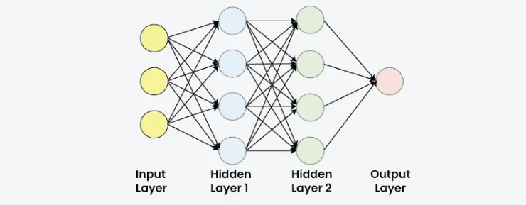 Think of it like building with Lego blocks: each block has a fixed role, and we stack them one on top of another to shape the final model. For example, let’s take a single Dense (Linear) layer. The pre-activation output is computed as:
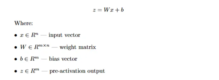
This is a weighted sum of the inputs plus a bias term—plain linear mathematics combining numbers. Then we apply an activation function (a non-linear function like ReLU, Sigmoid, or Tanh) to yield the layer output:

This non-linearity lets the model capture curves, twists, and complex patterns instead of just straight lines. To train it, a loss function for a regression problem is defined as:

The loss is simply a measure of "how wrong" the prediction is. We use the calculus chain rule to compute the gradient of the loss with respect to the weights:
 Then we update the parameters using gradient descent:

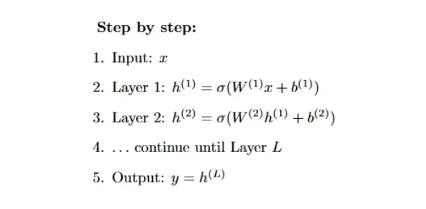
Picture this as nudging the weights bit by bit downhill until the network finds a sweet spot where errors are minimized. Ultimately, an explicit neural network can be represented as a composition of functions:

Where each layer is explicitly defined as:

Visualizing Explicit Stacking in PyTorch
import torch
import torch.nn as nn
import torch.optim as optim

class ExplicitNN(nn.Module):
    def __init__(self):
        super().__init__()
        self.lay1 = nn.Linear(3, 4)
        self.act1 = nn.ReLU()
        self.lay2 = nn.Linear(4, 1)

    def forward(self, x):
        x = self.lay1(x)
        x = self.act1(x)
        x = self.lay2(x)
        return x

# Synthetic Data Setup
x = torch.randn(5, 3)
y_true = torch.randn(5, 1)

model = ExplicitNN()
optimizer = optim.Adam(model.parameters(), lr=0.01)
criterion = nn.MSELoss()

# Explicit Trading Loop
for epoch in range(10):
    y_pred = model(x)
    loss = criterion(y_pred, y_true)
    optimizer.zero_grad()
    loss.backward()
    optimizer.step()
    print(f"Epoch {epoch+1}: Loss = {loss.item():.6f}")
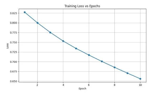 Over 10 epochs, the loss steadily decreases from 0.827 → 0.656, showing that the network is gradually learning the mapping from inputs to outputs. Each epoch represents a full pass through the data, where the model adjusts its weights slightly to reduce prediction errors. The smooth downward trend reflects the core idea of traditional neural networks: by explicitly computing outputs and backpropagating the errors, the network “nudges” itself closer to the target step by step. This incremental improvement is the hallmark of explicit, layer-by-layer learning.
While explicit layers are simple and intuitive, they have some limitations. Each layer computes outputs using a fixed formula, which can make modeling certain complex behaviors, like equilibrium states, constraints- difficult or inefficient. It’s like trying to capture the motion of a bouncing ball by stacking more and more Lego blocks: the more blocks you add, the heavier and clumsier the tower gets, yet you still don’t capture the true physics.
To represent patterns like these, we often end up stacking many layers, which eats up memory, slows down training, and sometimes still fails to express the system’s underlying rules. That’s where researchers asked: what if instead of telling the network step by step what to do, we just tell it the condition that must be satisfied and let it figure things out?
2. Implicit Layers So what exactly makes a layer ‘Implicit’?
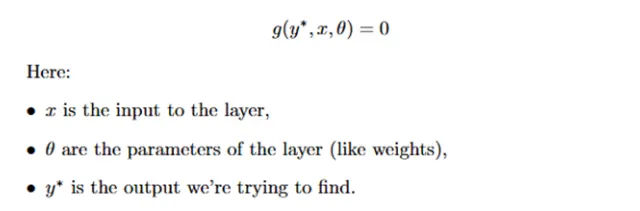
An implicit layer is different from the explicit layers we saw earlier because it doesn’t directly tell you how to compute the output. Instead, it defines the output as the solution to an equation. Formally, we say the output y* is whatever value satisfies:
Let’s look at some sample code to understand it better:class ImplicitLayer(nn.Module):
    def __init__(self, hidden_dim=4):
        super().__init__()
        self.W = nn.Linear(hidden_dim, hidden_dim)
        self.U = nn.Linear(3, hidden_dim)
        self.activation = nn.Tanh()


    def forward(self, x, tol=1e-4, max_iter=50):
        y = torch.zeros(x.size(0), self.W.out_features)
        norm_diffs = []


        for _ in range(max_iter):
            y_next = self.activation(self.W(y) + self.U(x))
            norm = torch.norm(y_next - y).item()
            norm_diffs.append(norm)
            if norm < tol:
                break
            y = y_next.detach()


        return y, norm_diffs


# Example usage
x = torch.randn(5, 3)
layer = ImplicitLayer()
y_star, norm_diffs = layer(x)


print("Equilibrium output y*:\n", y_star)
Equilibrium output y*:
 tensor([[-0.5969, -0.1887, -0.4900,  0.5574],
        [-0.5885,  0.3956,  0.7259,  0.8667],
        [-0.3710,  0.0120,  0.1901,  0.9733],
        [-0.5489,  0.6624, -0.0144,  0.3213],
        [-0.4723, -0.5047,  0.0988,  0.9635]])
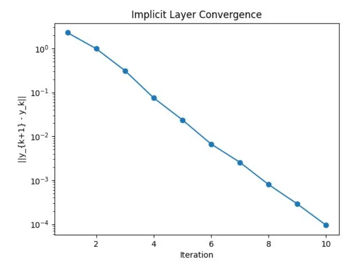 We see that, in contrast to the traditional Neural Network, the implicit layer doesn’t output values immediately. Instead, it iteratively “searches” for a solution that satisfies the fixed-point condition y∗ = f(y∗, x), y^* = f(y^*, x), y∗ = f(y∗, x).
Become a Medium member But all this just makes it seem like “Implicit Layers” is just making the whole process harder?- like why bother replacing a neat formula with something that requires solving an equation (multiple times!!). It’s because this unlocks a lot of benefits that explicit layers struggle with:
Infinite Depth without infinite parameters: Instead of stacking multiple layers on top of each other, we can attain an infinite layer model with just one layer’s worth of parameters. Memory Efficiency: Since we do not have to store every layer’s parameters and values, training can be done with MUCH lower memory. Built-in constraints and equilibria: Many real-world systems (physics, finance, biology) are naturally defined by equilibrium states or optimization constraints. Implicit layers let us model those directly, instead of approximating them with huge explicit stacks. From Implicit Layers to Deep Equilibrium Models (DEQs) Now here’s where things get exciting. One of the most powerful ways this idea has been applied is in Deep Equilibrium Models (DEQs).
DEQs take the concept of implicit layers and run with it: instead of building a very deep residual network by stacking identical layers again and again, they jump straight to the “equilibrium point” — the stable state you’d get if the network were infinitely deep.
In other words: a DEQ is like running an infinite ResNet, but solving directly for the end state instead of actually stacking infinite layers.
This idea is not just theoretical — researchers turned it into a powerful model called the Deep Equilibrium Model (DEQ).
- Deep Equilibrium Models (DEQs): The Infinite Network for the Price of One The concept of using a fixed-point equation as a layer is not just theoretical; it lays down one of the most exciting recent architectures: the Deep Equilibrium Model (DEQ): a “modern” variant of recurrent backpropagation.
To understand a DEQ, let’s start with the idea of repeated blocks in a deep network, like a Residual Network (ResNet). Imagine this network so deep that every single layer uses the same parameters θ (weight tying). To ensure the output depends on the input x, we add an input injection term (Ux) to every layer.
The network’s state update rule is

Press enter or click to view image in full size
This process is essentially modeling an infinitely deep network where the same layer is applied repeatedly.
The DEQ approach directly finds the point where this iteration stabilizes: the equilibrium point z∗. This fixed point is defined by the DEQ equation:

Press enter or click to view image in full size
The DEQ models an infinitely deep network while requiring only the parameters θ = {W, U, b} of a single function f.
Forward Pass: Solving the Puzzle with Speed To find the equilibrium z∗, we must use an iterative solver. While naive iteration zk + 1 = f(zk, x) is possible, Anderson Acceleration (AA) is the preferred method. AA is a quasi-Newton method that accelerates convergence by computing the next iterate.
zk+1 as a linear combination of previous iterates and function evaluations.
The forward solve happens outside the automatic differentiation (AD) tape within a torch.no_grad(): block. This is key to memory efficiency, as we avoid storing the computational graph and all temporary iterates created during the solve.
class DEQFixedPoint(nn.Module):
    def forward(self, x):
        with torch.no_grad():
            z_star, self.forward_res = self.solver(
                lambda z: self.f(z, x),
                torch.zeros_like(x)
            )

        z_out = self.f(z_star.clone().detach().requires_grad_(), x)

        return z_out
- The Backward Pass Secret: Implicit Differentiation The true power of DEQs lies in computing the gradient of the loss L with respect to the parameters θ (∂θ/∂L) efficiently, without running the backward pass through the unrolled solver.
The Theory: The Implicit Function Theorem (IFT) The IFT allows us to directly compute gradients at the solution point z∗. Starting with the fixed-point identity z∗=f(z∗, x, θ), we differentiate implicitly w.r.t θ:
 **
**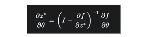
This formula depends only on the value of f and its derivatives at the final equilibrium point z∗.
Step 1: Solve a Linear Fixed-Point Equation for g
The backward pass first solves for the vector g (the incoming gradient transformed by the inverse transpose Jacobian). This is written as a linear fixed-point problem:

We solve for g iteratively using an efficient solver like AA. This step vastly improves memory consumption as no intermediate variables from the forward pass need to be stored
Step 2: Compute the Final Gradient
Once g is found, the final gradient ∂θ/∂L is computed as a single VJP operation:

The final DEQ module is built by implementing this logic with a backward hook on the output z, which triggers the linear solver only during the backward pass.
Implicit layers aren’t just theory — they’re powering real-world domains like quantitative finance.
- From DEQs to Derivatives: Implicit Layers in Quant Finance The implicit layer paradigm extends to another powerful class:
Differentiable Optimization (DiffOpt), where the output is defined as the solution to a minimization problem

This is highly relevant to quantitative finance, as many core problems are inherently optimization-based, such as Portfolio Optimization.
The Quant Advantage: Hard Constraints and KKT Conditions Enforcing Hard Constraints: Explicit layers approximate constraints (e.g., non-negative weights). DiffOpt layers, however, guarantee that the output. z∗ is the optimal solution to the strictly constrained problem (e.g., ∑zi=1).
KKT Conditions: For convex optimization problems common in finance (like Quadratic Programs), the optimal solution is defined by the Karush-Kuhn-Tucker (KKT) conditions. These KKT conditions form a system of nonlinear and linear equations/inequalities.
Differentiability via IFT: Similar to DEQs, the core idea in DiffOpt is to treat the KKT conditions as the implicit equation G(z∗, λ∗, ν∗, x, θ) = 0. Applying the IFT to these conditions allows us to compute the exact gradient.
Example: The Differentiable Quadratic Program (DQP)
The DQP forms the basis of Mean-Variance Portfolio Optimization.
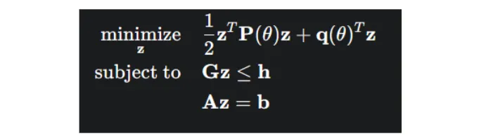
In this model, the risk P and return q are parameterized by a neural network’s weights θ. The DQP layer acts as a differentiable, constrained solver. This allows for End-to-End Learning, where the system learns the optimal predictive parameters θ such that the final constrained portfolio z∗ minimizes a top-level trading loss. The shift from explicit instructions to implicit conditions is changing deep learning. Whether by granting us infinite-depth capacity in DEQs while preserving O(1) memory, or by enabling the seamless integration of constrained financial optimization into end-to-end models, the Implicit Function Theorem is the single line of calculus that makes it all possible.
Implicit layers mark a significant revolution in deep learning — it is a shift from telling the networks what to do, to asking them to find the solution by satisfying the conditions given on their own. By framing the layers as equilibrium conditions or as optimization tasks, we can model infinitely deep behaviour, while using significantly less memory. Whether we are capturing complex dynamics or embedding constrained optimization in finance, Implicit layers open up a path towards networks that find reason and not just blindly compute.
The future of deep learning may no longer be about building deeper towers — but about finding deeper understanding within a single, self-consistent layer.
