
Options price Modeling is an exclusive skills of estimating the prices as well as volatility apart from just crunching numbers for giving the much accurate signals for the traded option under consideration.Modern day quant companies weights options as their knight among their instruments , where a good upper hand(better estimates) can 2x their profits.
If you are new to options : please check out the following blog for learning about options
While for a recap :
Options gives you the right, but not the obligation, to buy or sell an asset at a future date for a predetermined price.
Strike price : The value of the asset price at which the underlying asset will be bought or sold at the time of expiration.
What are we calculating inherently:
Suppose A and B have a contract between them for A selling his cycle to B after one month at 200(asset value). Now A is having some risk and some profit with this contract. But I now want to buy this option from B : So at what price should B sell me this contract , this price is called the fair value of the options. Which we will be calculating today….
Today we will move forward in the journey of options price modeling by exploring the journey from the Traditional methods and then we will look into its limitations based on the assumptions/ conditions .
In summary, the itinerary for our journey will be like
- Binomial model
- Black Scholes Merton Model
- Local Volatility (Dupire)
- Heston-LSV
For an in-depth understanding we will also look into the code of simulating the models for serving our purpose.
For simple understanding reference we will start with our stock(asset) is currently trading at 100$.
Intuitive “Binomial Model” or the two path model
Recall our example ,
In one month, we know it will either be 90 (down-state). We want to price a call option with a strike price of 100).

| Variable | Parameter | Value / Description |
|---|---|---|
| S₀ | Current Stock Price | 100 |
| K | Option's Strike Price | 100 |
| r | Risk-free Interest Rate | 5% |
| u | Up-factor | 1.2 (Price moves to 120) |
| d | Down-factor | 0.8 (Price moves to 80) |
Our goal is to find the option's price today, C`. We do this by working backward from the future.
Step 1: Find the Option's Payoff at Expiration
- Up State (Cu): If the stock goes to 20.
- Down State (Cd): If the stock goes to 0.
So, we know the option will be worth either 0. How do we value that uncertainty today?
Step 2: The Replicating Portfolio (The "Why")
The core idea is that we can build a portfolio of the underlying stock and risk-free bonds that has the exact same payoffs as the option.
- Portfolio in Up State = $20
- Portfolio in Down State = $0
By the "no-arbitrage" principle (you can't make risk-free money), the price of our option today must equal the cost of building this replicating portfolio today.
Step 3: Risk-Neutral Probability (The "How")
Solving the math for that replicating portfolio gives us a clever shortcut called "risk-neutral probability," or p.
This p is a synthetic probability. It's not the real chance of the stock going up. It's the probability we would need in a "risk-neutral" world to make the math work.
The Formula for p: This formula finds the probability p that makes the expected future stock price (discounted at the risk-free rate) equal to today's stock price.
p = (1+r) - d / u - d
- Our Calculation:
- p = (1 + 0.05) - 0.8 / 1.2 - 0.8
- p = 0.25 / 0.4 = 0.625
This means we'll use a 6.25% chance for the "up" move and a 37.5% (1-p) chance for the "down" move in our pricing.Step 4: Discount the Expected Payoff
Now, the option's price today (C`) is simply the expected future payoff (using our special p), discounted back to today at the risk-free rate.
The Formula for C`
C` = p * Cu + (1-p) * Cd / 1+r
- Our Calculation:
- C` = (0.625 * 0) / 1.05
- C` = 12.5 + 0 / 1.05
- C` ≈ $11.90
And that's it. The fair value of the option today is $11.90. This price is "fair" because it's the exact cost to build a portfolio that perfectly mimics the option's future, removing all risk.
Limitations :
The real world is not a simple two-path journey. A stock can take on thousands of potential prices. The model is too basic for reality.
The traditional “Black Scholes“

We will look into the black scholes model in a deep intuitive way, along with mathematical modeling so if we are confident about the heart strings of Black Scholes Model. You can skip to the later part but I wouldn't mind glancing this once.
Let us begin from our own intuitive approach of “Binomial” where the price could either move upward or downward and to approach realistic situations lets divide it into small timeframes. Instead of one big step over a month, what about two steps over two weeks? Or thirty steps over thirty days? Or millions of tiny steps every second?
Lets take this to ♾️ time intervals → The jagged lines turn down into smooth curves.
But how do we calculate the price of the option after small “dt” time interval ?
The mathematical limit of a that simple random decision to a simple random walk. It's a process Wt where the change over a tiny time dt is a random variable drawn from a normal distribution.
Well if we again recall it is not the stock price we made the decision for , but the returns it produced : So that the price doesn’t falls negative at any point.
(Stock price×(1+return))
This type of walk is mathematically termed as “Geometric Brownian Motion”
And the variable ‘Wt’ is termed as Random Variable of Weiner process.
But is that enough? Does it aligns to what actually market does?
We will try to break down this into two separate parts individually, (Expected Part) + (Unsteady Part)
Expectancy : Expected value of any random motion is given by ∑X*P(X) where P(X) is the probability of that price X.
Expected part = (μ*St).dt , where μ = (Expected price / Stock price )
σ (sigma) is the volatility, and dWt is the "tiny random step" from Brownian motion.
Unsteady part / Diffusion part : σStdWt
So, the tiny change in the stock price dSt is described by this continuous-time formula:
<p style="text-align:center;"> dSt= μStdt + σSt(dWt) </p>Because of this, the stock price at any future time T, ST, follows a Log-Normal Distribution.
🔍 How Do We Calculate the Option Price?
In the binomial world, we calculated the option price C by stepping backward one time step Δt from the end:
<p style="text-align:center;"> (Option price)C=e−rΔt [p⋅Cu+(1−p)⋅Cd] </p>We can't do that here; we have infinite steps. So, how do we find the option's price C which depends on both the stock price S and time t, written as C(S,t)?
We need a tool that tells us how C changes when S (which is random) and t (which is deterministic) both take one tiny step forward.
We need to take help from mathematics here : It's essentially the chain rule from calculus with two variables “t” and “stock price”, but should be able to handle the randomness of Brownian motion.
It gives us a formula for the tiny change in the option price, dC:

This can also be broken down into two terms :
- The dt part: The deterministic change.
- The dWt part: The random change in C caused by the stock's random "jiggle."
Create a risk-free portfolio.
- The Portfolio (Π): We construct a portfolio by shorting 1 option (−C) and longing Δ (Delta) shares of the stock (+ΔS).
(In binomial model) Δ=(Cu−Cd)/(Su−Sd) →(continuous world) Δ=∂S/∂C
- (dΠ): Change in the portfolio value over time dt
- Substituting the Brownian motion: Now lets substitute the stock price (from GBM) and dC (from chain rule) into that tiny dΠ equation.
To use the predicted stock price for our advantage , we chose our Δ perfectly so that the random dWt terms (the source of all risk!) exactly cancel each other out.
This leaves us with a portfolio whose change dΠ is completely deterministic :
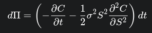
The No-Arbitrage Argument:
- Portfolio we have made is riskfree for small time interval dt. In a no-arbitrage world, any risk-free asset must earn the risk-free interest rate r.
- Therefore, the change in our portfolio dΠ must also equal the risk-free return on its value: dΠ=rΠdt.
- Since Π=ΔS−C=(∂S/∂C)S−C, we set our two expressions for dΠ equal:

- We just divide by dt & rearrange for famous Black-Scholes Partial Differential Equation (PDE):

Summary : This equation is the continuous-time version of the binomial model. It governs the price of any derivative on an asset following GBM. Solving this PDE (with the boundary condition C=max(ST−K,0) for a call option) is what gives us the final Black-Scholes formula for C(S,t).
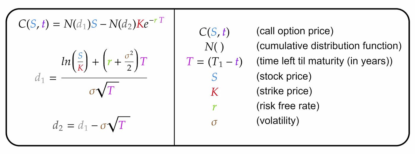
BSM provides a single yet elegant formula to price European-style options.
Limitations of Black-Scholes Model :
The market charges different “volatility prices” for different options. This directly contradicts the core assumption of Black-Scholes which assumes a constant volatility can be used for all options of the same stock. The first plot shows that Out-of-the-Money put options (low strike prices) have a higher implied volatility and Out-of-the-Money call options (high strike prices) have a lower implied volatility than the ATM strike price (taken here to be 100) which is the current stock price. The second plot shows the “smile pattern” in different volatility regimes.
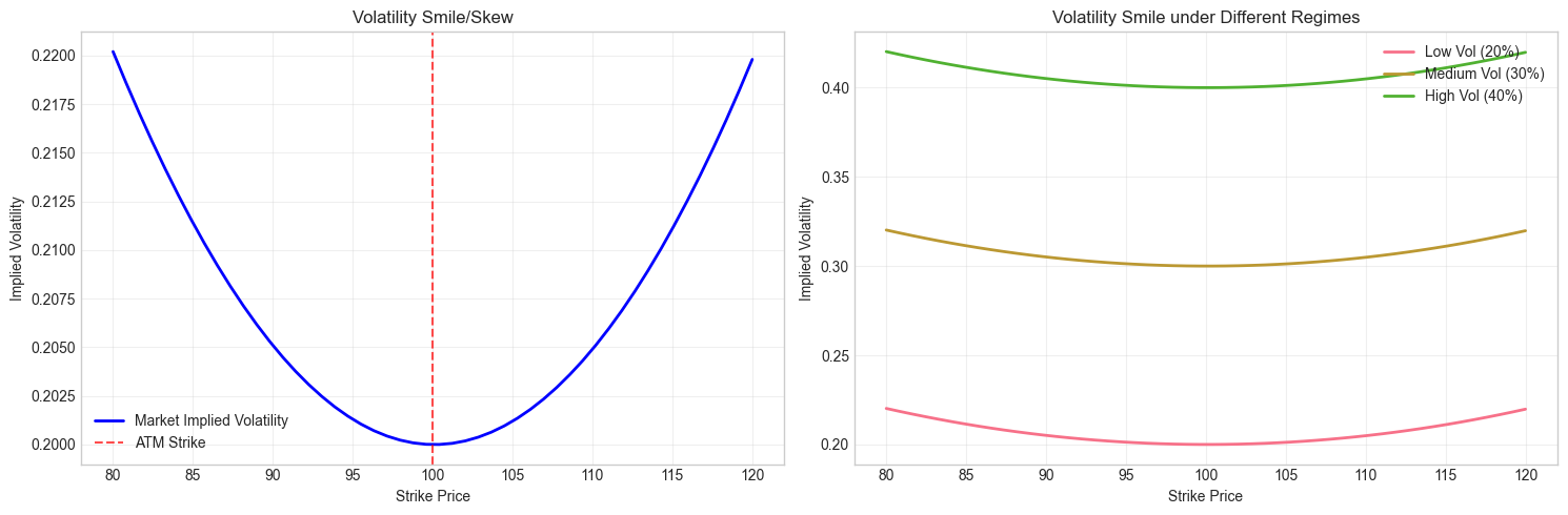
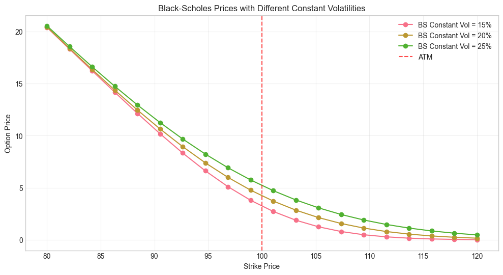
Observation: No single constant volatility can fit the entire volatility smile!
Local Volatility : Dupire Formula
The “smile 🙃” problem in the Black Scholes was solved by Dupire 🙂
Black-Scholes (BS): Assumes one constant σ and use the model (the Binomial tree or the PDE) to find the price C of one option. To learn more about the tree analogy , visit the Black-Scholes Section in our own blog pricing american options.
We know that σ (in real life) is not constant.While it depends on the stock price and the time.
This means our tree must be more flexible. At every single node (at each specific S and t), the "up" and "down" moves (and their probabilities) might be different. This is an Implied Tree.
Formulating “The local volatility “ :
Dupire's insight was to "flip" the variables. Instead of fixing the option (K,T) and asking how its price C changes with S and t, he did the opposite. He fixed the present (S0,t0) and asked how the option price C changes as we vary its contract terms: the strike K and the expiry T.
Now we are looking at the entire surface of C(K,T) ,that we see in the market. We converge to the equation from the Black Scholes PDE , where Stock price → particular Strike price.

Where q is the dividend yield (else 0 for simplifying)
“Aha moment” : Only unknown in this equation is 𝜎 (ie.volatility), so we get the market implied volatility.
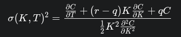
Dupire (LSV):
This is the "local volatility" function. It gives you the only volatility σ at a specific point in price-time space (S=K,t=T) that is consistent with the entire surface of market option prices. It's the continuous-time limit of the "implied tree" we built from scratch.
This σ(S,t) function can then be plugged back into the original Black-Scholes PDE to price any other derivative (like exotic options) consistently with the vanilla options market.
Assuming constant risk free rate ‘r’, the formula can be stated as:
<div class="flex justify-center my-6"> <img src="https://sohamagarwal.threnlabs.com/assets/qc_blog_images/image10.png" class="max-w-[90%] h-auto bg-white p-2 sm:p-4 rounded-md shadow-sm"> </div>Where ‘Wt’ is a Wiener process and ‘St’ is the current asset level.
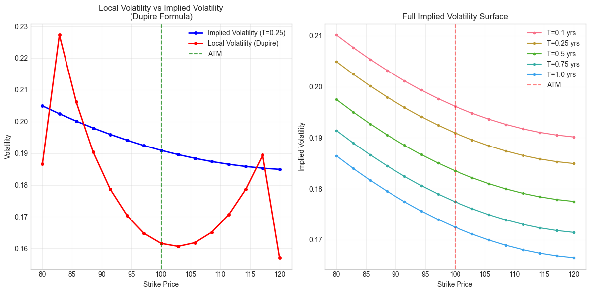
INTUITION: What Local Volatility Represents
==================================================
Local Volatility Interpretation:
ATM (K=100):
- Implied Vol: 19.094%
- Local Vol: 16.162%
→ If S_t reaches 100, use 16.162% vol for next step
OTM Put (K=85):
- Implied Vol: 20.012%
- Local Vol: 20.617%
→ If S_t crashes to 85, use 20.617% vol
OTM Call (K=115):
- Implied Vol: 18.583%
- Local Vol: 17.869%
→ If S_t rallies to 115, use 17.869% vol
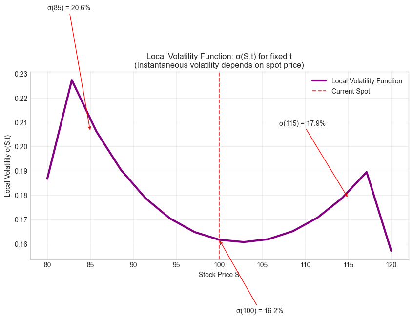
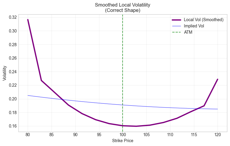
This graph has an ‘M’ shape due to the small second derivatives from discrete market data. In practice, a raw Dupire calculation is too unstable, thus smoothing becomes essential. A correct one using cubic splines for smooth derivative calculations, regularization to avoid division by small numbers, a Dupire plot should look something like this.
Monte Carlo Simulations
Monte Carlo simulations are simply just the repeated random sampling to compute numerical outcomes. They are employed in quantitative finance to simulate the stochastic (random) processes that underlie financial markets.By creating thousands or even millions of potential future situations for variables such as asset prices and volatilities, the approach enables us to estimate the distribution of possible outcomes, in place of a single determinate prediction.
In our case to simulate LSV, Monte Carlo simulations becomes necessary. The fundamental problem with the LSV approach is its condition of self-consistency:
the local volatility term, <img src="https://sohamagarwal.threnlabs.com/assets/qc_blog_images/image4.png" class="inline-block h-4 sm:h-5 align-middle mx-1.5 px-1 bg-white rounded-sm shadow-sm">, is a function of the conditional expectation of the stochastic variance, <img src="https://sohamagarwal.threnlabs.com/assets/qc_blog_images/image40.png" class="inline-block h-6 sm:h-8 align-middle mx-1.5 px-1 bg-white rounded-sm shadow-sm">, which in turn is a function of the paths generated based on <img src="https://sohamagarwal.threnlabs.com/assets/qc_blog_images/image4.png" class="inline-block h-4 sm:h-5 align-middle mx-1.5 px-1 bg-white rounded-sm shadow-sm">.
This introduces circular dependence that cannot be broken analytically. Thus, Monte Carlo method is the computational core that translates the LSV model from theoretical idea to working pricing and risk management instrument.
Heston LSV Model :
The local volatility model assumes volatility is a deterministic function of the underlying asset price and time. This contradicts empirical evidence that volatility itself is random and fluctuates over time (stochastic). It fails to capture the "volatility of volatility."
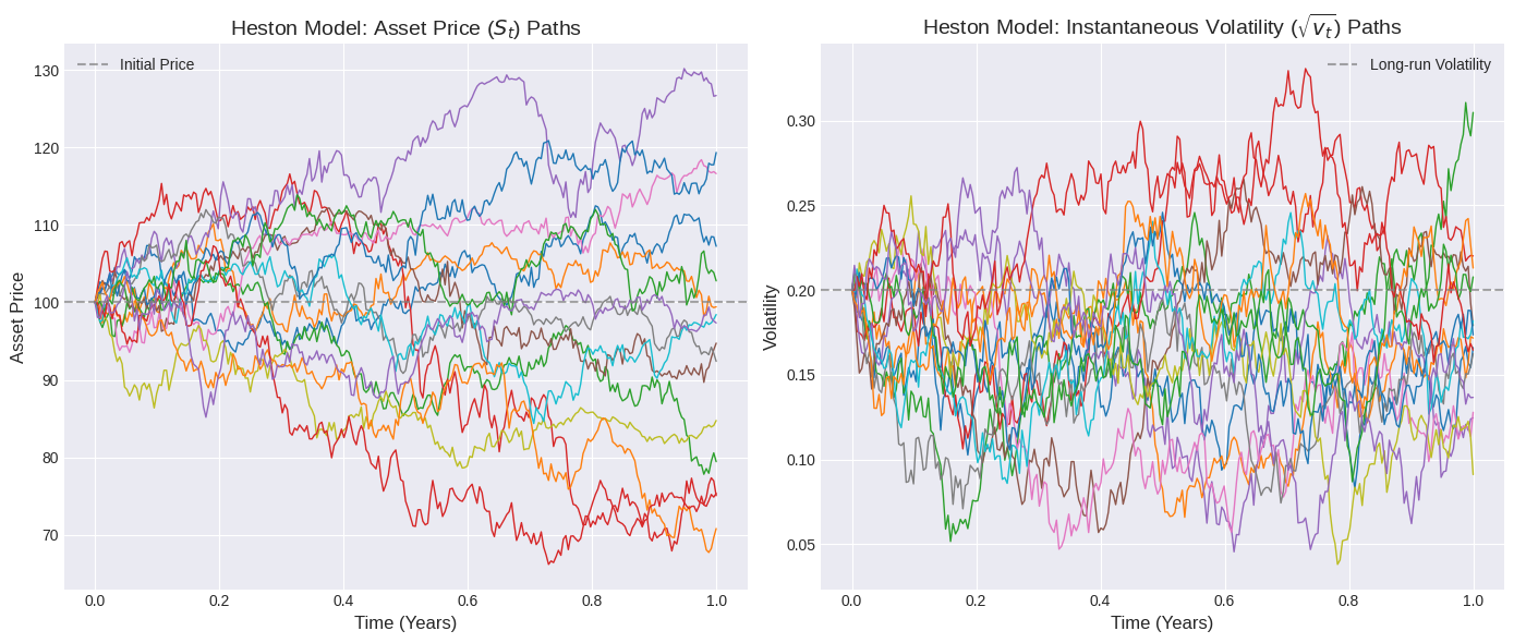
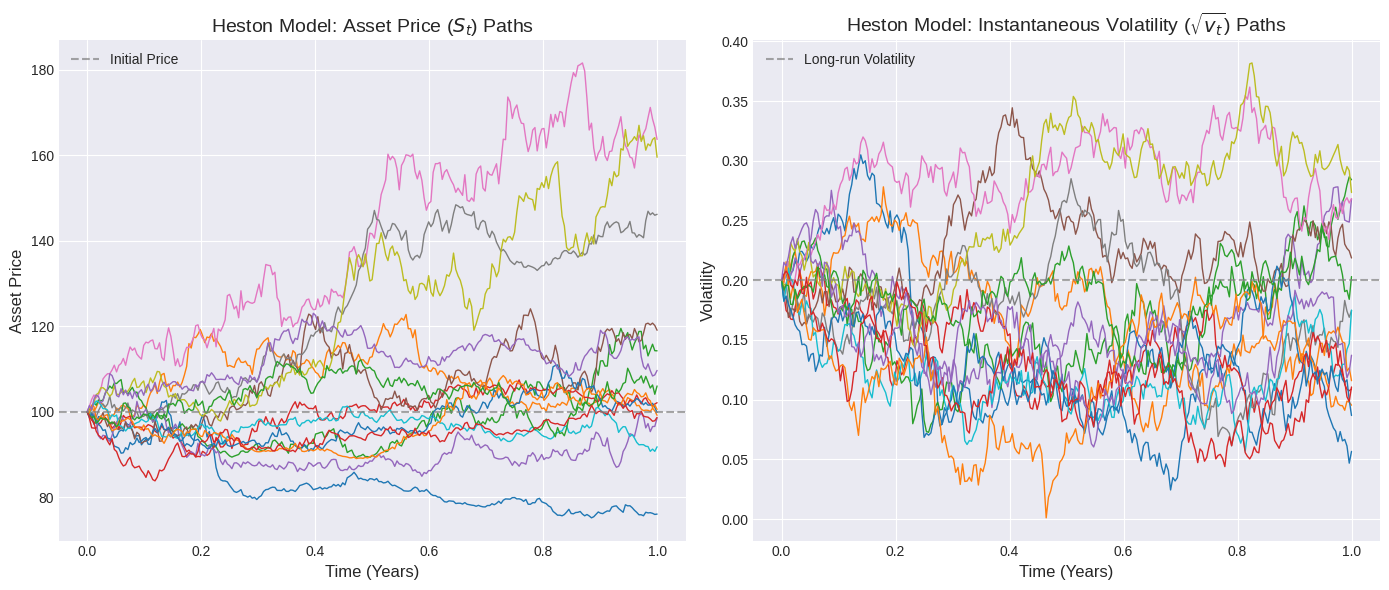
The Heston model introduces stochastic volatility by modeling the variance (volatility squared) as a separate stochastic process. This means that volatility itself can change randomly, mirroring real-world market behavior. By explicitly modeling stochastic volatility, the Heston model naturally generates the implied volatility smile and skew, and more importantly, it provides a dynamic framework for how this smile evolves over time. The correlation between the asset price and its volatility, a key parameter in Heston, directly drives the skew.
Simulation Implication:
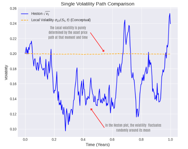
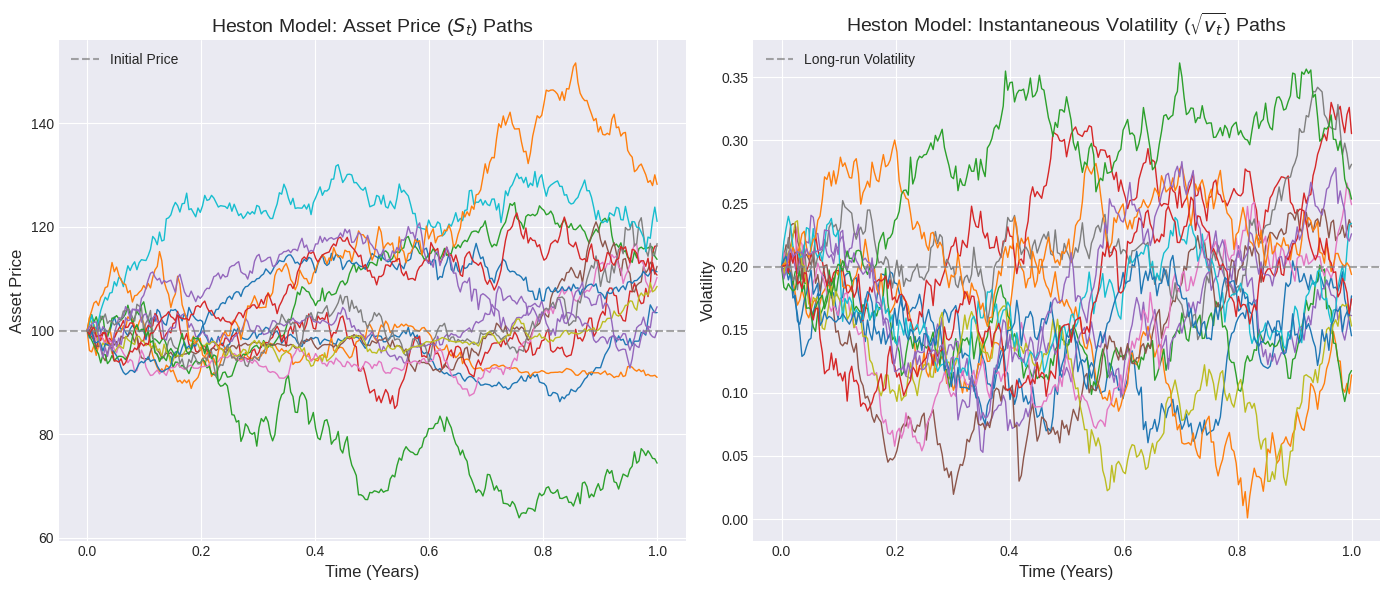
In a Monte Carlo simulation of the Heston model, you would see the simulated volatility paths fluctuating over time, rather than being fixed by the asset price and time as in local volatility. This allows for more realistic option pricing and risk management.


Are the systems of stochastic differential equations used for the Heston Model. Where dW1,t and dW2,t are Wiener processes with correlation ρ, i.e., E[dW1,tdW2,t]=ρdt
Parameters :
- μ: Asset drift (e.g., the risk-free rate r)
- V_t: Instantaneous variance
- κ: Rate of reversion of v_t to θ
- θ: Long-run mean variance
- σ: Volatility of volatility (vol-of-vol)
- ρ: Correlation between S_t and v_t
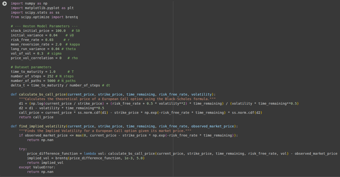
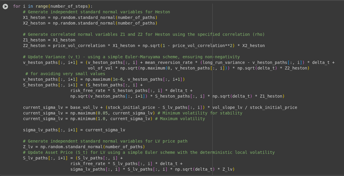
For solving the SDE’s , we use numerical schemes like the Euler scheme here for Δt time step , each for Asset Price(S) and variance(v) , finally turning out into..


Code
Let’s prepare a program to visualize them..👀
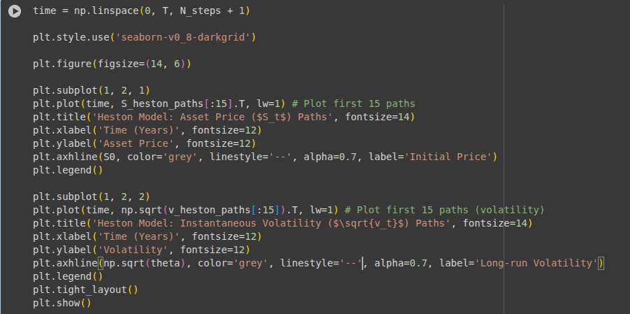
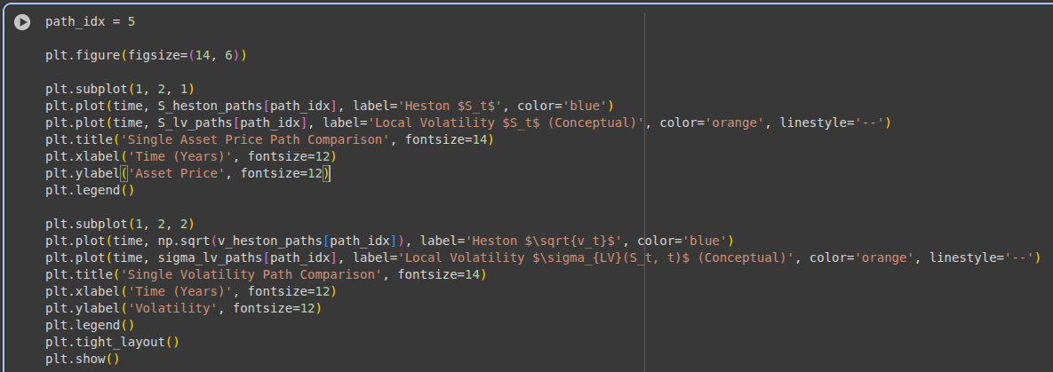
Results
<div style="display: flex; justify-content: center;"> <img src="https://sohamagarwal.threnlabs.com/assets/qc_blog_images/image7.png" alt="Description 1" style="width: 49%; margin-right: 1%;" /> <img src="https://sohamagarwal.threnlabs.com/assets/qc_blog_images/image46.png" alt="Description 2" style="width: 49%; margin-left: 1%;" /> </div> <p style="clear: both;"></p> <!-- Add this to clear the float for subsequent content -->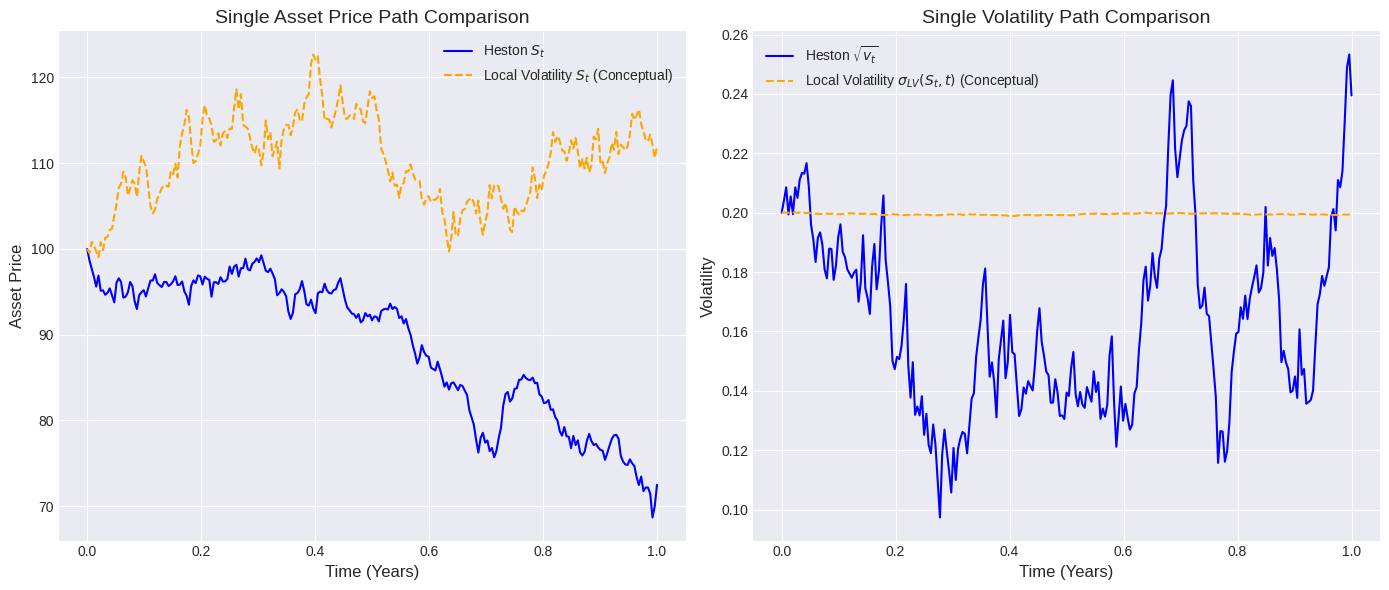
Example
Imagine you are trying to price a call option on a stock. With our original example….
Current Stock Price (S): $100
Current Time (t): Today
Expiration Time: 3 months from now
Using an "LV Path" Model
Using the Heston Model
The statement says: "If two LV paths hit the same (S,t), their subsequent volatility MUST be the same.
"This means if, at any point in the future, two different simulated paths of the stock price happen to reach a specific price of, say, $105 at one month from now, then the model forces the future volatility for both those paths to be identical from that point onwards.
The statement says: "In Heston, two paths could hit the same (S,t) but have different v(t) values, leading to different future volatilities."
The Heston model is a stochastic volatility model, meaning it models volatility itself as a random process. So, even if two simulated paths of the stock price reach the exact same stock price (S) at the exact same time (t), their associated volatility (v(t)) at that moment could be different. This difference in current volatility would then lead to different future volatility paths and, consequently, different option prices.
Path A: Stock goes from 105 in 1 month, then to $110 in 2 months.
Path B: Stock goes from 105 in 1 month, then to $95 in 2 months.
According to the LV model, at the 1-month mark when both paths hit 105 might have been different.
Path A: Stock goes from 105 in 1 month, with its associated volatility (v(t)) being, say, 20%.
Path B: Stock goes from 105 in 1 month, but its associated volatility (v(t)) is, say, 30%.
Even though both paths are at $105 at the 1-month mark, the Heston model allows for them to have different levels of volatility at that point. This difference in current volatility (20% vs. 30%) will mean their future volatility movements will likely diverge, leading to different expected future stock price distributions and thus different option prices..
- volatility was assumed to be constant for LV model
- If two LV paths hit the same (S,t), their subsequent volatility MUST be the same.
- Heston Model accounts for the volatility of “Volatility”
- In Heston, two paths could hit the same (S,t) but have different v(t) values, leading to different future volatilities.
In essence:
- LV models tie future volatility directly to the current stock price and time. If you know (S,t), you know future volatility.
- Heston models introduce an additional dimension of randomness for volatility. Knowing (S,t) isn't enough; you also need to know the current volatility state at (S,t) to project future volatility
.
Dependence on Rho(⍴) :
| Correlation | Volatility Skew | Implication |
|---|---|---|
| For rho < 0 | Volatility Skew (smile skewed to the left, higher implied vol for OTM puts) | Implies a "leverage effect" (stock prices and volatility are negatively correlated – when prices drop, volatility tends to increase) |
| For rho > 0 | Volatility Skew (smile skewed to the right, higher implied vol for OTM calls) | Implies that volatility increases when prices rise (less common in equity markets, more in commodities) |
| For rho = 0 | Symmetrical Volatility Smile | No correlation between asset price and volatility |
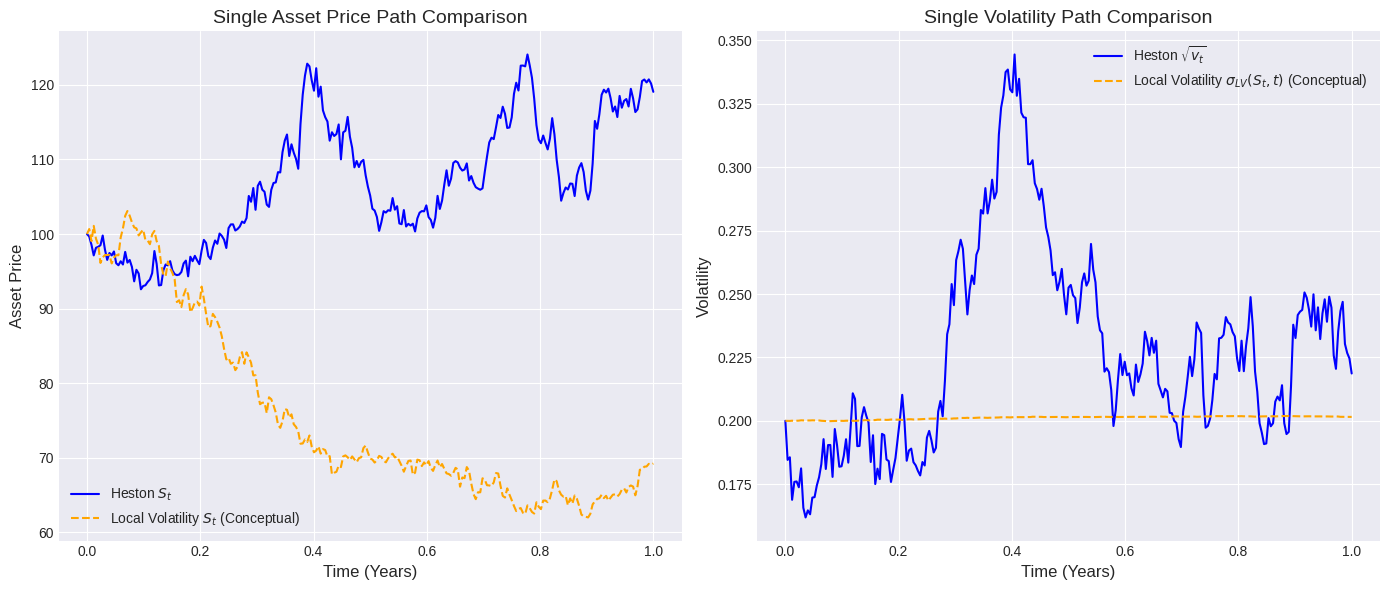
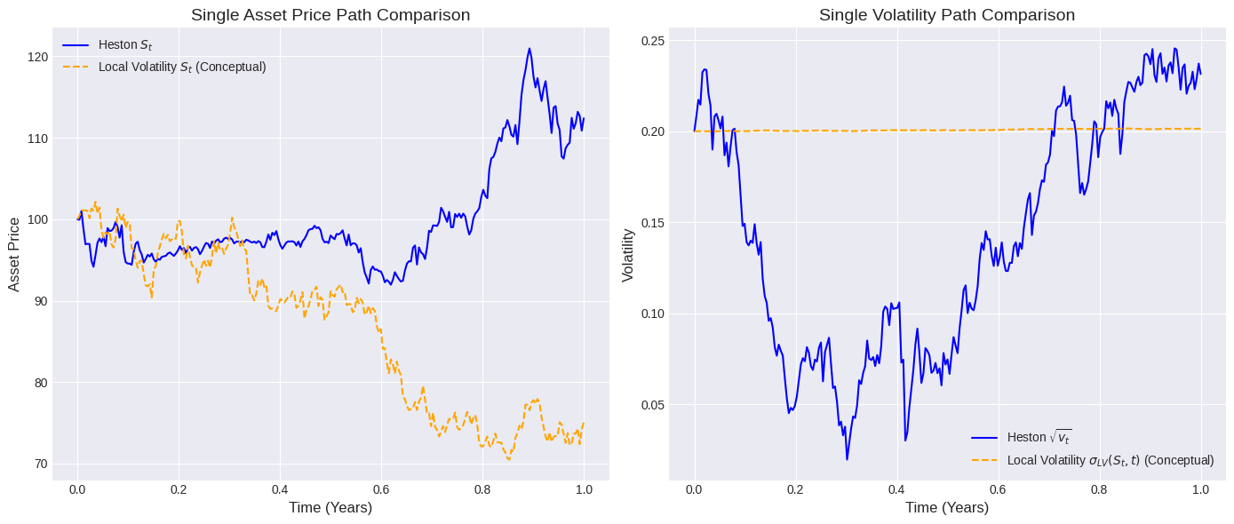
It tends to have better out-of-sample predictive capabilities. Its parameters (mean reversion, long-term variance, vol-of-vol, correlation) are more fundamental to market behavior. Where Local Volatility model struggles with out of sample options (options with different maturities or strikes than training data).
Heston LSV Model - Monte Carlo Simulation
The fundamental limitation of the Heston Model is its inability to perfectly fit the entire volatility surface with a small number of parameters.
<div style="display: flex; justify-content: center;"> <img src="https://sohamagarwal.threnlabs.com/assets/qc_blog_images/image43.png" alt="Description 1" style="width: 33%; margin-right: 1%;" /> <img src="https://sohamagarwal.threnlabs.com/assets/qc_blog_images/image37.png" alt="Description 2" style="width: 33%; margin-left: 1%;" /> <img src="https://sohamagarwal.threnlabs.com/assets/qc_blog_images/image45.png" alt="Description 2" style="width: 33%; margin-left: 1%;" /> </div> <p style="clear: both;"></p>The heston model creates a parametric volatility surface that may not match market prices exactly, especially for short-dated options or extreme strikes.
By running the heston model on three sets of parameters:
| Mean Reversion (κ) | Long-term Var (θ) | Vol of Vol (ξ) | Correlation (ρ) | Initial Var (v₀) |
|---|---|---|---|---|
| 2.0 | 0.04 | 0.3 | -0.7 | 0.04 |
| 1.5 | 0.045 | 0.4 | -0.8 | 0.05 |
| 3.0 | 0.035 | 0.25 | -0.6 | 0.03 |
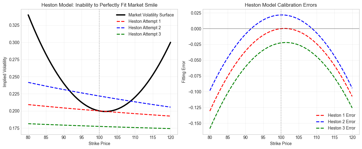
We can show that a single set of parameters is unable to accommodate the market volatility surface.
This is where the Heston-LSV model improves. It introduces a local volatility component that enables perfect fit for the current volatility surface while maintaining realistic dynamics. The first statement of the Heston model can be rewritten as: <img src="https://sohamagarwal.threnlabs.com/assets/qc_blog_images/image26.png" class="inline-block h-6 sm:h-8 mx-1 align-middle px-1 bg-white rounded-sm"> The calibration condition ensures perfect fit: <img src="https://sohamagarwal.threnlabs.com/assets/qc_blog_images/image28.png" class="inline-block h-6 sm:h-8 mx-1 align-middle px-1 bg-white rounded-sm"> Something to be noted is that this model has infinite degrees of freedom through <img src="https://sohamagarwal.threnlabs.com/assets/qc_blog_images/image8.png" class="inline-block h-5 sm:h-6 mx-1 align-middle px-1 bg-white rounded-sm">, while maintaining the stochastic volatility dynamics.
<div class="my-10 bg-[#0d1117] rounded-xl border border-white/10 overflow-hidden shadow-2xl"> <div class="flex items-center justify-between px-4 py-2 bg-white/5 border-b border-white/10"> <div class="flex gap-1.5"> <div class="w-2.5 h-2.5 rounded-full bg-red-500/60"></div> <div class="w-2.5 h-2.5 rounded-full bg-amber-500/60"></div> <div class="w-2.5 h-2.5 rounded-full bg-emerald-500/60"></div> </div> <span class="text-xs font-mono text-gray-400">heston_lsv_calibration.py</span> </div> ```python print("\n2. Demonstrating Heston-LSV Perfect Calibration") def heston_lsv_calibration(market_iv, heston_iv, E_v_given_S): # Under Heston-LSV, we can achieve perfect fit by adjusting sigma_LSV sigma_dupire = market_iv # Simplified assumption sigma_lsv = sigma_dupire / np.sqrt(E_v_given_S)# Verify calibration: sigma_lsv^2 * E[v|S] should equal sigma_dupire^2
verified_iv = sigma_lsv * np.sqrt(E_v_given_S)
return sigma_lsv, verified_iv
Simulate conditional expectation (typically from Heston dynamics)
E_v_given_S = 0.04 + 0.01 * (K - 100) / 100 # Linear approximation
Calculate required LSV component
sigma_lsv, calibrated_iv = heston_lsv_calibration(market_iv, heston_iv, E_v_given_S)
</div>
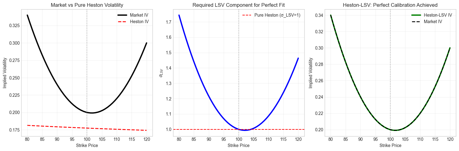
As shown by the code snippet and graphs above, the Heston-LSV is able to achieve perfect calibration against Market IV.
Dynamics Preservation: The Fundamental Advantage
Dupire’s local volatility model can fit the volatility surface, but has unrealistic dynamics.
- Predicts flattening volatility smiles in the future
- Forward volatility behaviour does not match market observations
- Sticky-strike v/s Sticky-delta behaviour is incorrect
Heston model provides realistic dynamics
- Mean-reverting volatility matches empirical observations
- Persistent volatility smiles in the future
- Correct forward volatility behaviour
- Realistic spot-volatility correlation leverage effect
Heston-LSV combines the best of both worlds:
- Perfect static fit to current volatility surface
- Realistic future dynamics from stochastic volatility
#### A Monte-Carlo simulation of this model:
<div class="my-10 bg-[#0d1117] rounded-xl border border-white/10 overflow-hidden shadow-2xl">
<div class="flex items-center justify-between px-4 py-2 bg-white/5 border-b border-white/10">
<div class="flex gap-1.5">
<div class="w-2.5 h-2.5 rounded-full bg-red-500/60"></div>
<div class="w-2.5 h-2.5 rounded-full bg-amber-500/60"></div>
<div class="w-2.5 h-2.5 rounded-full bg-emerald-500/60"></div>
</div>
<span class="text-xs font-mono text-gray-400">heston_lsv_mc.py</span>
</div>
```python
def heston_lsv_monte_carlo(S0, v0, r, kappa, theta, xi, rho, sigma_lsv_func, T, n_steps, n_paths, scheme='full_truncation'):
dt = T / n_steps
S_paths = np.zeros((n_paths, n_steps + 1))
v_paths = np.zeros((n_paths, n_steps + 1))
sigma_lsv_paths = np.zeros((n_paths, n_steps + 1))
# Initialize paths
S_paths[:, 0] = S0
v_paths[:, 0] = v0
sigma_lsv_paths[:, 0] = sigma_lsv_func(S0, 0) # Initial LSV component
# Cholesky decomposition for correlated Brownian motions
L = np.array([[1, 0], [rho, np.sqrt(1 - rho**2)]])
for i in range(1, n_steps + 1):
t = (i-1) * dt # Current time
# Generate correlated random numbers
Z = np.random.normal(size=(n_paths, 2))
Z_corr = Z @ L.T
# Get current state
S_prev = S_paths[:, i-1]
v_prev = v_paths[:, i-1]
sigma_lsv_prev = sigma_lsv_paths[:, i-1]
# Discretize variance process based on chosen scheme
if scheme == 'full_truncation':
# Full truncation: v_prev is used in drift, max(0,v_prev) in diffusion
v_next = v_prev + kappa * (theta - np.maximum(v_prev, 0)) * dt + \
xi * np.sqrt(np.maximum(v_prev, 0)) * np.sqrt(dt) * Z_corr[:, 1]
v_paths[:, i] = np.maximum(v_next, 0)
elif scheme == 'reflection':
# Reflection: take absolute value of variance
v_next = v_prev + kappa * (theta - v_prev) * dt + \
xi * np.sqrt(np.abs(v_prev)) * np.sqrt(dt) * Z_corr[:, 1]
v_paths[:, i] = np.abs(v_next)
elif scheme == 'partial_truncation':
# Partial truncation: v_prev in drift, max(0,v_prev) in diffusion
v_next = v_prev + kappa * (theta - v_prev) * dt + \
xi * np.sqrt(np.maximum(v_prev, 0)) * np.sqrt(dt) * Z_corr[:, 1]
v_paths[:, i] = np.maximum(v_next, 0)
else:
raise ValueError("Scheme must be 'full_truncation', 'reflection', or 'partial_truncation'")
# Get LSV component at current spot and time
sigma_lsv_current = np.array([sigma_lsv_func(s, t) for s in S_prev])
sigma_lsv_paths[:, i] = sigma_lsv_current
# Total volatility: sigma_LSV * sqrt(v)
total_vol = sigma_lsv_current * np.sqrt(np.maximum(v_prev, 0))
# Euler discretization for stock price (log-space for better stability)
S_paths[:, i] = S_prev * np.exp(
(r - 0.5 * total_vol**2) * dt +
total_vol * np.sqrt(dt) * Z_corr[:, 0]
)
return S_paths, v_paths, sigma_lsv_paths
Final price stats: mean=101.56, std=16.22 Final vol stats: mean=0.182, std=0.045 Simulating: Constant LSV = 1.0 (Pure Heston)
Results
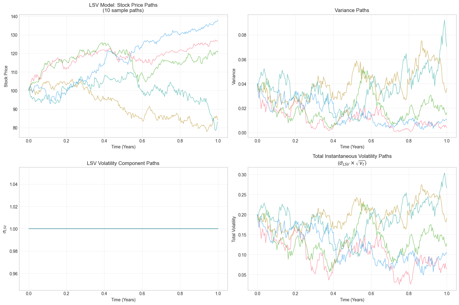
Final price stats: mean=103.67, std=16.65 Final vol stats: mean=0.177, std=0.046
Simulating: Time-decay LSV
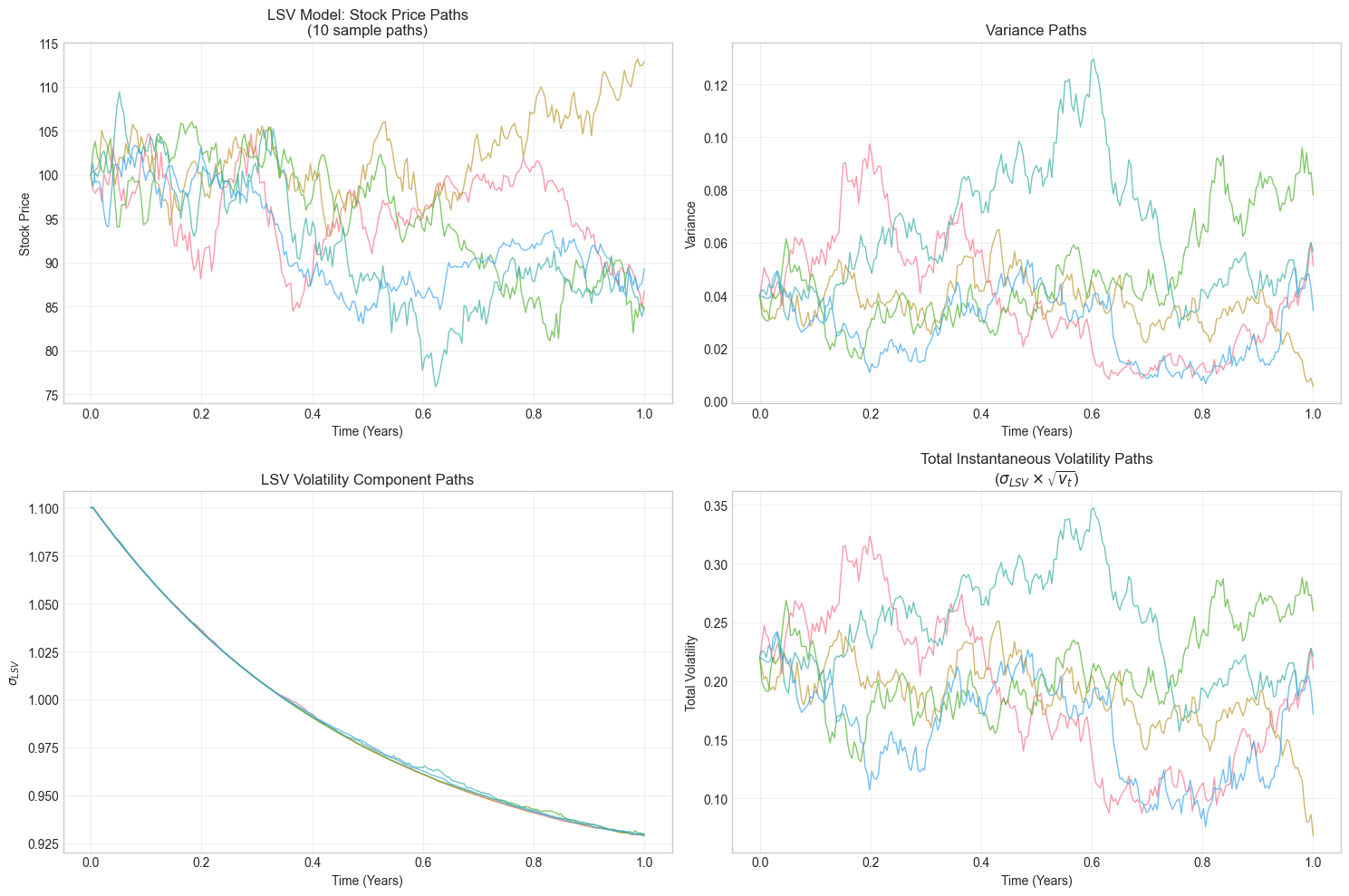
Final price stats: mean=91.68, std=10.70 Final vol stats: mean=0.186, std=0.065
- The first graph of each case shows simulated price evaluation under LSV dynamics. The paths fan out due to stochastic volatility and exhibit realistic drift with occasional large moves from the local volatility component.
- Graph 2 displays the stochastic volatility process - paths mean-revert around long-term variance θ but with persistent deviations, showing the volatility clustering effect.
- 3rd Graph is the <img src="https://sohamagarwal.threnlabs.com/assets/qc_blog_images/image4.png" class="inline-block h-4 sm:h-5 align-middle mx-1.5 px-1 bg-white rounded-sm shadow-sm"> function along each path, plotted against time. It is constant in the first case (Pure Heston dynamics) and a smile that flattens towards the future in case of time decay (more realistic).
- The final graph for the simulation shows the combined effect <img src="https://sohamagarwal.threnlabs.com/assets/qc_blog_images/image4.png" class="inline-block h-4 sm:h-5 align-middle mx-1.5 px-1 bg-white rounded-sm shadow-sm"> × √v ; paths demonstrate realistic volatility dynamics with both mean reversion and spot-dependent adjustments.
Find closest time indices
time_indices = [np.abs(time_axis - t).argmin() for t in time_points]
fig, axes = plt.subplots(2, 3, figsize=(18, 10))
Plot 1: Conditional expectation of variance at different times
for i, (t, idx) in enumerate(zip(time_points, time_indices)): S_t = S_paths[:, idx] v_t = v_paths[:, idx]
# Bin by stock price and compute conditional expectation
S_bins = np.linspace(np.percentile(S_t, 5), np.percentile(S_t, 95), 15)
bin_indices = np.digitize(S_t, S_bins)

E_v_given_S = []
S_centers = []
for j in range(1, len(S_bins)):
    mask = (bin_indices == j)
    if np.sum(mask) > 5:
        E_v_given_S.append(np.mean(v_t[mask]))
        S_centers.append(np.mean(S_t[mask]))
</div>
Advanced Analysis: LSV Model Properties
---
Running comprehensive LSV analysis...
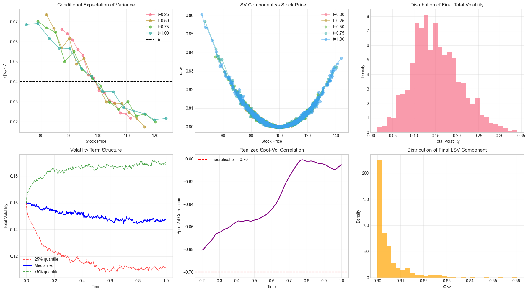
- The first graph shows how expected variance changes depending on stock price- typically higher for lower prices (due to leverage effect).
- 2nd graph shows how the local volatility function <img src="https://sohamagarwal.threnlabs.com/assets/qc_blog_images/image44.png" class="inline-block h-6 sm:h-8 align-middle mx-1.5 px-1 bg-white rounded-sm shadow-sm"> varies over different stock levels. Forms inverse curve because calibration requires <img src="https://sohamagarwal.threnlabs.com/assets/qc_blog_images/image4.png" class="inline-block h-4 sm:h-5 align-middle mx-1.5 px-1 bg-white rounded-sm shadow-sm"> to compensate where conditional variance is extreme.
- The 3rd graph is the histogram of final instantaneous volatilities showing the range and concentration of outcomes. This forms a skewed distribution because stochastic volatility creates right-tailed outcomes from volatility clustering.
- The 4th plot shows evolution of volatile quantiles over time, showing how volatility uncertainty changes with horizon. This forms converging bands because mean reversion pulls extreme volatilities towards long term mean over time.
- 5th graph Shows actual correlation between stock returns and volatility changes over time v/s theoretical
<img src="https://sohamagarwal.threnlabs.com/assets/qc_blog_images/image11.png" class="inline-block h-4 sm:h-5 align-middle mx-1.5 px-1 bg-white rounded-sm shadow-sm">. Forms a noisy line around theoretical <img src="https://sohamagarwal.threnlabs.com/assets/qc_blog_images/image11.png" class="inline-block h-4 sm:h-5 align-middle mx-1.5 px-1 bg-white rounded-sm shadow-sm"> because Monte-carlo paths exhibit the leverage effect with sampling variation.
- The final graph shows histogram of final <img src="https://sohamagarwal.threnlabs.com/assets/qc_blog_images/image4.png" class="inline-block h-4 sm:h-5 align-middle mx-1.5 px-1 bg-white rounded-sm shadow-sm"> values showing how much the local volatility component varies across paths. Forms concentrated distribution because <img src="https://sohamagarwal.threnlabs.com/assets/qc_blog_images/image4.png" class="inline-block h-4 sm:h-5 align-middle mx-1.5 px-1 bg-white rounded-sm shadow-sm"> is a smooth function, but varies across different price regions.
Conclusion to the Blog:
Throughout this three-part journey, we’ve unraveled the story of Local-Stochastic Volatility models, moving from foundational concepts to hands-on application. We started by exploring why the usual models fall short: Black-Scholes clings to a constant volatility, local volatility models can behave unrealistically, and even Heston’s approach struggles with calibration. Against this backdrop, the LSV framework stood out as a smart and practical solution, offering both a strong market fit and realistic forward-looking behavior.
As we delved into the math using Fokker-Planck equations, we uncovered an elegant self-consistency condition at the core of LSV calibration:
<div class="flex flex-wrap justify-center items-center gap-2 my-8 text-xl font-medium">
<img src="https://sohamagarwal.threnlabs.com/assets/qc_blog_images/image39.png" class="h-8 align-middle bg-white px-1.5 py-0.5 rounded shadow-sm">
<span class="text-white">² × 𝔼[v|S] = </span>
<img src="https://sohamagarwal.threnlabs.com/assets/qc_blog_images/image5.png" class="h-8 align-middle bg-white px-1.5 py-0.5 rounded shadow-sm">
<span class="text-white">²</span>
</div>
This insight turns a tough problem into something we can actually solve using fixed-point iteration. By building and running our own numerical models—from simulating Monte Carlo paths to estimating conditional expectations—we saw firsthand both the strengths and the real-world challenges of this approach.
While the road from mathematical theory to robust implementation presents numerical challenges - from derivative estimation artifacts to convergence stability - the LSV model stands as the current pinnacle in volatility modeling. It successfully resolves the fundamental tradeoff between perfect static calibration and realistic dynamic behavior, making it the preferred framework for exotic derivatives pricing, risk management, and volatility strategy development in quantitative finance.
## Summary:
The stock price can be affected by the following reasons
- Stock Price
- Current price of that stock
- Affected by volatility of that stock
- Strike Price :
- Leads to volatility curve /smirk
- The Time left for expiration of the stock.
