Nature-Inspired Optimization: Lighting Up Financial Markets with the Firefly Algorithm

Nature-inspired algorithms are very powerful and fascinating tools in optimization. They extract details about the working of biological systems and turn those rules into algorithms, which are good at finding solutions in messy, non-smooth and high-dimensional problems.

Can nature teach us how to model financial markets? In this blog, we dive into how bio-inspired algorithms can help us to tune time series models. We will explore why they matter and how they might be very relevant in this context, how they work, what problems they solve and how we used one of them—the Firefly Algorithm by Xin-She Yang, to estimate a GARCH-type volatility model.

Why Nature-Inspired Search for Financial Data?

Financial time series—like stock returns, commodity prices, volatility, etc.—are messy by nature. They are noisy, non-linear, and often non-stationary. You’ll find very odd and asymmetric clusters and spikes. Classical optimizers like gradient-based methods work neatly when the likelihood surface is smooth and easy—but financial data rarely is. In rugged and error-heavy likelihood surfaces, such optimizers can get stuck in local optima, slow down, or even fail altogether as complexity and dimensions rise.

Nature-inspired algorithms bring some advantages for these problems which can be very ideal for such chaotic scenarios:

• They handle non-linearity and complexity very 'naturally': They are often designed to explore and exploit such complex high-dimensional spaces.
• Global Optimization Focus: Instead of getting stuck on a local solution like traditional methods, bio-inspired algorithms use various mechanisms like adaptation and interaction etc. to jump out of this case and continue to find better solutions.
• Gradient-Free: They do not rely on gradients and derivatives, which might be computationally very expensive in certain scenarios.
• Flexibility: They provide good and clean ways to do feature selection and model tuning and hence are flexible.

Meet the Fireflies: Diving into the Firefly Algorithm

Before other various methods came into picture, the world of bio-inspired optimization was ruled by Particle Swarm Optimization (PSO) (Kennedy & Eberhart, 1995), a clever algorithm inspired by swarm behavior using randomness and internal communication among the particles. In PSO, each particle moves around the search space remembering its personal best and is pulled towards the swarm’s global best. It’s creative and powerful, but its global best pull can make the swarm converge too early, missing out on better, unexplored regions.

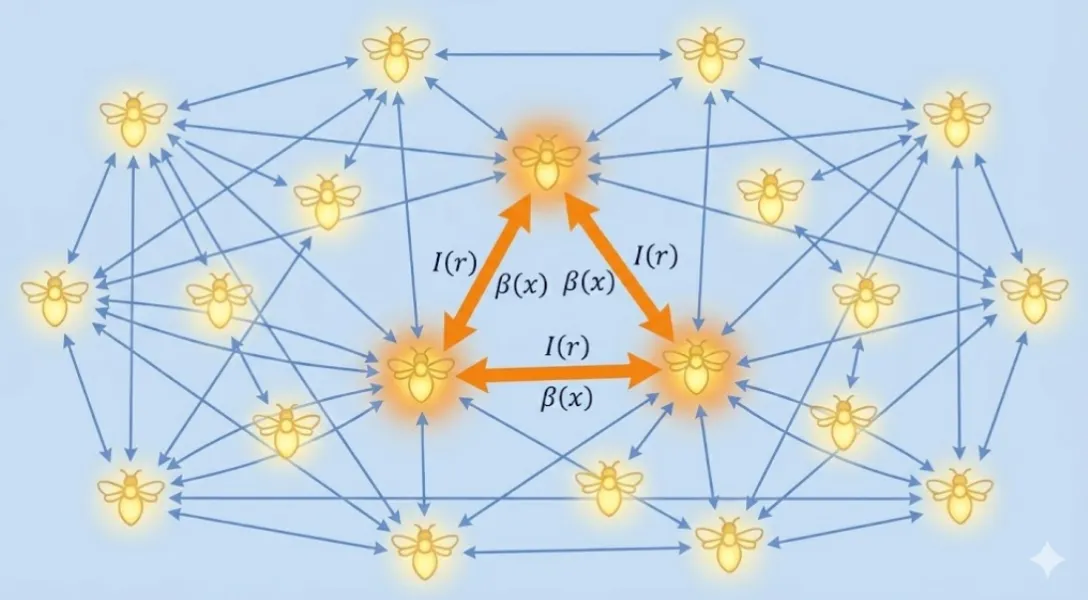
The rhythmic beautiful flashing light pattern of fireflies generally observed at night is an amazing phenomenon to witness. Each firefly in the group flashes, the brighter ones attract the dimmer ones. But since light fades with distance, multiple groups of fireflies form around different bright spots.

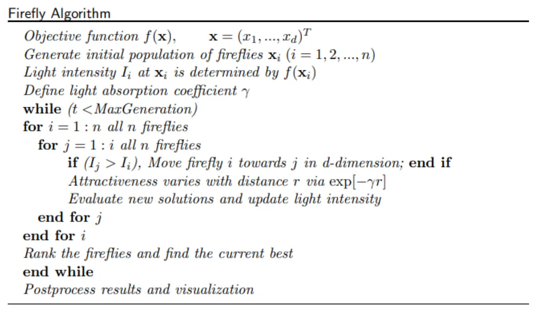
That’s the main idea behind the Firefly Algorithm (FA), which treats the flashes as optimization rules and uses many agents to search for a good solution at once in a clean way.

The Three Simple Rules in FA:

1. Any firefly can be attracted to any other—no extra conditions or restrictions.
2. Brighter fireflies attract dimmer ones—the darker one will move near the brighter one and the pull weakens with distance.
3. Better the firefly’s position, the brighter it shines. In optimization terms: brightness = the objective function value, i.e., $I(x)$ is directly proportional to $f(x)$:

In FA, the attractiveness is linked to their objective function value and the decay pattern of the attractiveness with distance. In nature, light gets weaker with distance and additionally it is absorbed by the medium too (e.g., air fog).

We know ideally in simplest form, light intensity $I(r)$ varies according to the inverse square law.

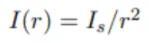
For a given medium with an absorption coefficient $\gamma$, the light intensity varies with distance $r$ as:

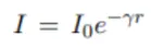
where $I_0$ is the original light intensity. The combined effect of the inverse square law and the absorption is often approximated as:

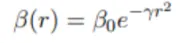
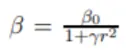
As a firefly’s attractiveness is proportional to the light intensity seen by the adjacent fireflies, we define a new term called the 'attractiveness' $\beta$ of a firefly by:

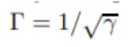
This also brings another term, the characteristic distance $r_g = \frac{1}{\sqrt{\gamma}}$. If two fireflies are separated by about this distance, the attraction has dropped to roughly $1/e$ times of its maximum.

If a function is required which decreases at a slower rate, we can also use the approximation:

Distance and Movement

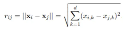
Distance between any two fireflies $i$ and $j$ at vectors $x_i$ and $x_j$ respectively is simply the Cartesian distance:

The movement of a firefly $i$ out of attraction towards the more brighter firefly $j$ is formulated as:

Interpretation:

• Directed Pull Term: In the second term of the RHS, $x_i$ is shifted toward a better vector $x_j$, so $i$ learns from $j$’s better fit.
• Distance Weighing Term: If $x_j$ is far away, its influence is small; this preserves multiple groups exploring different possible optimal answers. $\gamma$ characterizes the variation of attractiveness and is very important in determining the speed of convergence.
• Random Term: Exploration to avoid stationarity. $\alpha$ is the randomization parameter.

What Are We Doing with FA and Time Series?

Imagine your time series model as a machine with a bunch of knobs. One knob controls how fast volatility reacts to shocks, another controls how long shock persists and other knobs tweak other parameters similarly. If you set the knobs right, the machine will predict the wild ups and downs of the financial data; if not, it will break down.

GARCH-X Equation Employed:

The FA algorithm is our gradient-free way of finding those knob settings. Each firefly is one unique complete set of knob settings. We let these fireflies loose. They test their settings against history, generate forecasts, and get “brighter” if their settings produce less surprise (lower Negative Log Likelihood) which is a better fit.

Fireflies fly toward brighter fireflies and show aggregate behavior. They also wiggle randomly. Over many generations, the swarm concentrates around the brightest optimal configuration estimate.

How We Lit the GARCH-X Model: Implementation Details and Tweaks Used

We conducted our experiment on various stock’s daily data from 2017 to 2024. Instead of looking at simple closing prices, we computed Parkinson’s Volatility, and used it as the volatility proxy using the daily High and Low prices, capturing intraday spikes/crashes that the standard close-to-close data misses. If $H_i, L_i$ are the High and Low prices respectively for each period $i$, then the Parkinson’s volatility estimate is given by the equation:

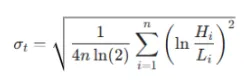
We implemented a custom GARCH-X recursion that models the log variance. We fed it our Parkinson’s proxy as an external signal, allowing the model to react to intraday volatility signals immediately.

Financial markets have fat tails; crashes happen more often than a normal distribution predicts. We used the Student-t distribution likelihood, allowing the Firefly Algorithm to learn exactly how “heavy” the tails are (finding degrees of freedom roughly 4).

To keep parameter guesses rational and avoiding any subsequent blowup, we scaled each quantity by appropriate factors or either transformed them, and all external inputs were z-scored (rolling window) to prevent the optimizer to be biased towards features with larger magnitudes and let our Firefly algorithm converge faster.

After computing the fitted volatility, we then validated the model using walk-forward cycles:

• Cycle 1: Training on 2017–2022 $\rightarrow$ Forecasting 2023
• Cycle 2: Training on 2017–2023 $\rightarrow$ Forecasting 2024

We then plotted the visual plots and analyzed the MSE and Quasi Likelihood.

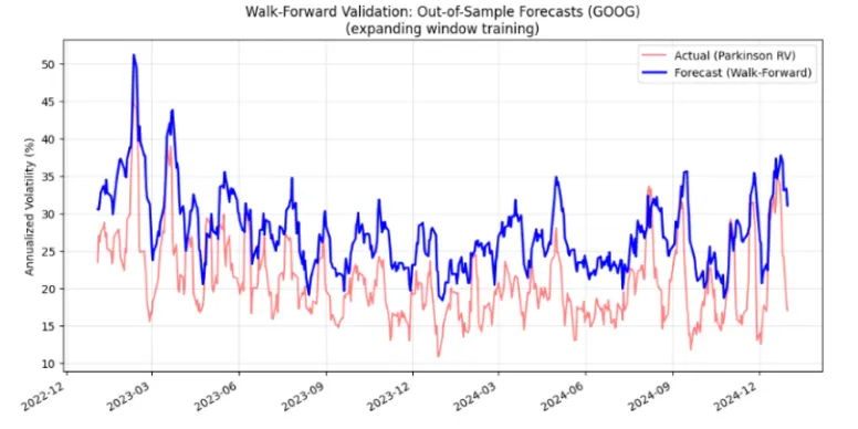
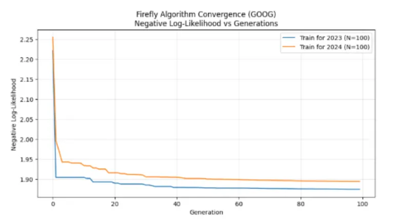
OOS Forecast Results on GOOG (2023–2024)

Code Implementation

Below is the basic implementation of the firefly optimization function with a stochastic update mechanism:

import numpy as np
import numpy.random as npr
import math

def firefly_opt(func, dim, pop=40, gens=200, alpha0=0.6, alpha_decay=0.995, beta0=1.0, gamma_vis=0.5, subset_j=10, seed=2025):
    rng = npr.default_rng(seed)

    # initialize population using a previously written initialization function and their objective value
    population = init_population(pop, dim, seed=seed)
    objectives = np.array([func(population[i]) for i in range(pop)], dtype=np.float64)

    best_idx = int(np.argmin(objectives))
    best_solution = population[best_idx].copy()
    best_obj = float(objectives[best_idx])

    history = [best_obj]
    alpha = alpha0

    if pop <= 1:
        return best_solution, best_obj, history

    for gen in range(gens):
        # randomizing update order each time
        order = rng.permutation(pop)

        for i in order:
            # picking a subset
            m = min(subset_j, pop-1)
            # choosing other indices
            other_indices = [k for k in range(pop) if k != i]
            chosen = rng.choice(other_indices, size=m, replace=False)

            for j in chosen:
                # if j is better, move
                if objectives[j] < objectives[i]:
                    rij = np.linalg.norm(population[i] - population[j])
                    beta = (beta0) * (math.exp(-gamma_vis * (rij**2)))
                    attraction = (beta) * ((population[j] - population[i]))
                    random_step = (alpha) * ((rng.random(dim) - 0.5))

                    # final
                    population[i] = (population[i] + attraction + random_step)

                    # evaluate new position immediately
                    val = func(population[i])
                    objectives[i] = val

                    # checking, updating global best
                    if val < best_obj:
                        best_obj = float(val)
                        best_solution = population[i].copy()

        # decay for convergence
        alpha = (alpha) * (alpha_decay)
        history.append(best_obj)

    return best_solution, best_obj, history

Important Practical tweaks used: Parameter mapping: to keep GARCH-X parameters valid in sensible ranges and to avoid the fireflies to go absolutely wild as they initially did unmapped. Exogenous regressors (Volume, RV) are rolling window Z-scored so the gamma coefficients are comparable to other parameters, and the returns are scaled by 10,000 to ensure it is on the same numeric scale. We mapped the raw vector through smooth functions:

This mapping keeps alpha + beta < 1 a requirement for the GARCH model.

The degree of freedom in the T distribution was mapped using a sigmoid function that ensures fat tails while keeping it > 2 which is required for finite variance. This keeps it in [2, 30].

The estimated log variance is also clipped in the interval [-10, 10] and constants are added, to prevent domain issues and issues due to very large values.

Smart Swarm initialization: the firefly population is initialized with gaussian noises, and the conditional variance path is not started at zero, instead it is initialized near the variance of the estimation window which ensures the convergence path starts at a somewhat realistic base level.

Firefly movement tweaks: We used a periodic decay factor for the attractiveness parameter: alpha to make the exploration slower gradually and make the algorithm converge sensibly without blowing up.

Stochastic updates: each firefly compares only to a random subset rather than all others which reduces the computation’s time which was earlier indefinite.

Conclusion This work was a fun intersection of two broad domains: biologically inspired models and financially time series modelling. We let a swarm of fireflies search for the perfect fit of GARCH-X parameters, until the model best fitted the market behavior.

Along the way , there were many serious challenges-such as instability from exploding variances, arbitrarily large values of the Likelihood function, extremely slow convergence, which made us slightly refine our approach with parameter mapping, sensible initialization etc. each tweak was useful and bought the model closer to stability, convergence and meaningful volatility forecasts.

This work shows that bio-inspired optimization has scope of meaningfully explaining financial models, a bridge between nature’s patterns and market complexity.

The glow of the fireflies is a reminder that even in noisy, chaotic data, intelligent search can still find very fundamental order and structure.