Navigating Wall Street with Reinforcement Learning: Teaching Machines to Trade

Let’s talk about the stock market. For most of us, it’s a mysterious beast. You buy a stock, it goes down. You sell it, it moons. It feels like the universe has a personal vendetta against your wallet. Traditional trading often relies on analysts who stare at charts until the squiggly lines start to look like their spirit animal, or on complex rules that shatter the moment the market sneezes.

(Press enter or click to view image in full size)

But what if you could teach a machine to trade? Not by just throwing in a dusty rulebook, but by allowing it to learn as it gathers experience, in a way an ordinary human would.

Enter Reinforcement Learning (RL), the same tech that powers AI that can beat grandmasters at Go and master video games. Now, it’s putting on a pinstripe suit and heading to Wall Street.

Real-Life Examples: Who’s Using the RL Secret Weapon?

When billions are on the line, you don’t use basic algorithms. You use RL, primarily in two critical areas:

• Optimal Execution: This is about buying or selling massive blocks of stock without telling the whole market what you’re doing (which would move the price against you).
• Dynamic Portfolio Management: Constantly adjusting thousands of assets to keep risk and returns perfectly balanced.

Major firms using or pioneering RL techniques include:

• Goldman Sachs & J.P. Morgan: They use RL agents for Optimal Trade Execution. The agent learns the best way to slice a huge trade into tiny parts and execute them over time to minimize cost.
• The Big Quants (e.g., Renaissance Technologies, Two Sigma): These secretive hedge funds use sophisticated Deep RL to discover new, subtle trading strategies and manage their multi-billion dollar portfolios with minute-by-minute efficiency.

The concept is even familiar in pop culture! Remember in The Big Bang Theory when Sheldon Cooper used reward-based feedback (chocolate) to modify Penny’s behavior? Trading firms are applying that same core principle — learning the optimal action through trial and error — to make billions in the stock market.

RL in a Nutshell: Agents, Environments, Rewards — The Survival Guide

If the trading challenge is the battlefield, Reinforcement Learning is the training academy. At its core, RL is remarkably simple: it’s how an Agent learns the best way to behave in a complex Environment by chasing Rewards. Think of it as training a very smart, greedy digital dog.

(Press enter or click to view image in full size)

[Image of reinforcement learning feedback loop agent environment action reward]

1. The Agent (The Trader)

The Agent is the Learner and the Decision-Maker. In trading, this is your AI algorithm.

• Role: To observe the market, decide the next action (Buy, Sell, Hold), and try to maximize its total long-term wealth.
• The Big Question: What do I do next?

2. The Environment (The Market)

The Environment is everything the Agent interacts with. In trading, this is the market itself — the prices, volatility, volume, and news.

• Role: To present the Agent with a current State (e.g., “The stock price is $100 and volatility is high”) and to react to the Agent’s action (e.g., if the Agent Buys, the price might tick up).
• The Big Question: What is happening now?

3. The Action (The Trade)

An Action is the choice the Agent makes.

• Role: The specific move the Agent executes at a given time. This can be discrete (Buy / Sell / Hold) or continuous (Buy $X\%$ of my portfolio / Sell $Y$ of my shares).
• The Big Question: How does my choice affect the environment?

4. The Reward (The Feedback)

The Reward is the crucial feedback loop — it’s the score the Agent receives immediately after taking an action. This is the RL equivalent of a pat on the head or a rolled-up newspaper.

• Role: To tell the Agent if the action was good or bad. In trading, the reward isn’t usually just “Did the stock go up?” — it’s about Risk-Adjusted Profit.
• Positive Reward: Portfolio value increases while maintaining a low drawdown.
• Negative Reward (Penalty): High transaction costs or sudden, dangerous volatility exposure.
• The Big Question: Did I do a good job?

The Learning Loop (Policy)

(Press enter or click to view image in full size)

The Agent’s ultimate goal is to develop an optimal Policy ($\pi$) — a set of rules that tells it the best action to take for every possible state of the environment.

The magic is that the Agent learns the best policy through billions of these trial-and-error iterations, constantly updating its strategy to maximize the total, long-term reward. This is how it learns to “survive” and thrive in the volatile financial environment.

RL Meets Wall Street: How It Powers Trading Strategies

Reinforcement Learning (RL) skips the guesswork. Instead of predicting the price, it focuses on the optimal action right now — Buy, Sell, or Hold — to maximize wealth over the long run. It’s like teaching a chess grandmaster to play the stock market.

The core problem RL solves is sequential decision-making under uncertainty. RL isn’t trying to predict the future; it’s learning the best way to react to it.

The Problem: The Market is Chaos Theory’s Playground

The stock market is not a mere simple math problem. It’s a gigantic multiplayer game being driven by logic, fear, greed, and breaking news. Just having an “if the price drops by 5%, sell!” strategy is like trying to navigate a maze with your eyes closed. You’re going to hit a wall. Fast.

RL is perfect for this kind of chaos because it does not need a rigid rulebook. It learns by doing. It makes a decision (buy, sell, or hold), sees the result of its action (gain or loss), and based on that outcome, it fixes how it makes that decision. This is the action-consequence cycle.

Our algorithm starts out completely clueless. It might buy at the peak and sell at the bottom, losing a ton of virtual money. But it learns. After thousands, or even millions, of simulated trading days, it starts to connect the dots. It begins to understand which market patterns (the ‘state’) are more likely to lead to a reward if it takes a certain action.

The Math Behind the Magic: Bellman Equations, Value Functions & the Policy Puzzle

Behind every smart AI is an elegant mathematical framework. For Reinforcement Learning, that framework tells our agent how to think, learn, and make decisions. Let’s move past the surface and look at the engine underneath.

The Core Components

First, let’s formally define the pieces of our trading puzzle:

• State ($s$): A snapshot of the market at a moment in time. This is a collection of data points like the current price, trading volume, and technical indicators (e.g., RSI, MACD).
• Action ($a$): A decision our agent can make (Buy, Sell, or Hold).
• Reward ($R$): An immediate numerical feedback for an action.
• Policy ($\pi$): The agent’s strategy. The policy, denoted as $\pi(a \mid s)$, tells us the probability of taking action $a$ when in state $s$.

Evaluating the Game: Value Functions

The immediate reward is nice, but what we really care about is the total future reward. Value functions estimate the long-term goodness of a situation.

1. The State-Value Function: $V^{\pi}(s)$

This function answers the question: “Starting from this state ($s$), what is the total reward I can expect if I follow my current strategy ($\pi$)??”

It’s defined as the expected return, which is the sum of all future rewards, discounted by how far away they are. The discount factor, $\gamma$ (gamma), represents patience — it makes immediate rewards more valuable than distant ones.

(Press enter or click to view image in full size)

$V^{\pi}(s) = \mathbb{E}_{\pi} \left[ \sum_{k=0}^{\infty} \gamma^k R_{t+k+1} \mid S_t = s \right]$

The $\mathbb{E}_{\pi}[\dots]$ part means we’re taking an average over all the possible future paths the market could take, given we’re following our policy $\pi$.

2. The Action-Value Function: $Q^{\pi}(s, a)$

This answers: “If I’m in this state ($s$) and I take this specific action ($a$), what is the total reward I can expect from then on?” This is the Q-function, and it’s a measure of how good a particular action is in a given situation.

(Press enter or click to view image in full size)

$Q^{\pi}(s, a) = \mathbb{E}_{\pi} \left[ \sum_{k=0}^{\infty} \gamma^k R_{t+k+1} \mid S_t = s, A_t = a \right]$

The Q-function is incredibly useful because if we know the Q-value for every possible action, the choice becomes simple: just pick the action with the highest Q-value!

The Recursive Masterpiece: The Bellman Equation

Calculating those long sums of future rewards is computationally impossible. This is where Richard Bellman’s brilliant insight comes in. The Bellman Equation provides a recursive relationship for value functions. It states that the value of your current state is the immediate reward you get, plus the discounted value of the next state you end up in.

For the State-Value function, the Bellman Expectation Equation is:

(Press enter or click to view image in full size)

$V^{\pi}(s) = \sum_{a} \pi(a \mid s) \sum_{s'} P(s' \mid s, a) \left[ R(s,a,s') + \gamma V^{\pi}(s') \right]$

In plain English: “The value of a state today is the average of the immediate reward plus the discounted value of whatever state comes next, assuming we follow our policy.”

Solving the Puzzle: Finding the Optimal Policy

We don’t want to just evaluate a policy; we want to find the best possible policy, called the optimal policy ($\pi^*$). This policy has a corresponding optimal value function, $V^*(s)$, and optimal action-value function, $Q^*(s, a)$.

To find these, we use the Bellman Optimality Equation. Instead of taking an average based on our policy, we greedily choose the best possible action at every step.

(Press enter or click to view image in full size)

$Q^*(s, a) = R(s, a) + \gamma \sum_{s'} P(s' \mid s, a) \max_{a'} Q^*(s', a')$

This equation is the heart of most RL algorithms. The optimal policy, $\pi^*$, is then simply to take the action that maximizes the optimal Q-function:

(Press enter or click to view image in full size)

$\pi^*(s) = \arg\max_{a} Q^*(s, a)$

This is exactly what an Actor-Critic agent tries to do. The Critic learns to estimate the value function ($V(s)$), and the Actor updates its policy ($\pi(a \mid s)$) in the direction suggested by the Critic, slowly but surely moving towards the optimal policy.

The PPO Principle: Taking Smart, Stable Steps

We have our Actor-Critic duo, where the Actor makes trades and the Critic provides feedback. But a crucial question remains: how should the Actor use that feedback? If the Critic signals a huge loss, should the Actor panic and completely change its strategy overnight? In the chaotic world of stock trading, such a drastic reaction is a recipe for disaster.

This is the exact problem Proximal Policy Optimization (PPO) is designed to solve.

The Danger of Unstable Learning

Imagine teaching someone to drive. If they drift slightly to the right, you don’t tell them to jerk the wheel all the way to the left. A small, gentle correction is what’s needed. Standard reinforcement learning algorithms can sometimes be like that panicky passenger, demanding a massive update to the Actor’s policy after a single mistake.

This can lead to a “destructive update,” where one bad lesson makes the agent forget all the good things it previously learned. PPO prevents this by encouraging the agent to take small, sensible steps — to behave less like a rookie gambler and more like a seasoned professional who cautiously increases their stake.

PPO’s Solution: Small Steps in a “Trust Region”

PPO is built on a simple yet powerful idea: the agent should only trust its strategy to be reliable within a small range of its current behavior. Therefore, any updates to the policy must be kept within a “trust region,” preventing the new strategy from straying too far from the old one.

This “baby steps” approach creates the perfect balance between:

• Exploitation: Sticking with strategies it knows already work.
• Exploration: Cautiously trying new, slightly different strategies to find an even better approach.

How PPO Stays on Leash: The Clipping Mechanism

So, how does PPO enforce this “small steps” rule? It uses a clever trick called clipping:

1. Calculate a Ratio

First, PPO calculates a probability ratio, $r_t(\theta)$, that asks: “How much more (or less) likely is our new policy to take this action compared to the old policy?”

(Press enter or click to view image in full size)

$r_t(\theta) = \frac{\pi_{\theta}(a_t \mid s_t)}{\pi_{\theta_{\text{old}}}(a_t \mid s_t)}$

If $r_t(\theta) > 1$, the new policy favors the action more. If $r_t(\theta) < 1$, it favors it less.

2. Multiply by the Advantage

Next, this ratio is multiplied by the Advantage ($A_t$), which is the Critic’s feedback. The Advantage tells us if the action was better ($A_t > 0$) or worse ($A_t < 0$) than the average expectation.

3. Apply the Clip

To stop the policy from changing too aggressively, PPO “clips” the ratio $r_t(\theta)$ within a narrow range, typically $[0.8, 1.2]$. Let’s call this range $[1-\epsilon, 1+\epsilon]$, where $\epsilon = 0.2$. The final objective PPO maximizes is:

(Press enter or click to view image in full size)

$L^{\text{CLIP}}(\theta) = \hat{\mathbb{E}}_t \left[ \min\left(r_t(\theta)\hat{A}_t, \text{clip}(r_t(\theta), 1-\epsilon, 1+\epsilon)\hat{A}_t\right) \right]$

This elegant mechanism has a powerful effect:

• When an action is GOOD ($A_t > 0$): We want to increase its probability. The clipping at $1+\epsilon$ prevents us from getting too greedy. The policy update is capped.
• When an action is BAD ($A_t < 0$): We want to decrease its probability. The clipping at $1-\epsilon$ prevents us from overreacting and slashing the probability to near zero after one bad trade.

Anatomy of the Code

Note: This code does serious number-crunching. It will take a standard machine around 20–25 minutes to run through the training phase.

1. Technical Indicator Computation

Technical indicators are mathematical formulas applied to historical price and volume data to help identify trends, momentum, and volatility. We calculate four widely-used indicators:

• MACD (Moving Average Convergence Divergence): Measures trend direction and momentum.
• RSI (Relative Strength Index): Gauges whether a stock is overbought ($>70$) or oversold ($<30$).
• CCI (Commodity Channel Index): Detects cyclical trends in price.
• ADX (Average Directional Index): Quantifies the strength of a trend.

def getdata(tickers, startdate, enddate):
    dataset = {}
    for ticker in tickers:
        stockdf = yf.download(ticker, start=startdate, end=enddate)
        stockdf['MACD'] = ta.macd(stockdf['Close'], fast=12, slow=26, append=True)['MACD_12_26_9']
        stockdf['RSI'] = ta.rsi(stockdf['Close'], length=14, append=True)
        stockdf['CCI'] = ta.cci(stockdf['High'], stockdf['Low'], stockdf['Close'], length=14, append=True)
        stockdf['ADX'] = ta.adx(stockdf['High'], stockdf['Low'], stockdf['Close'], length=14, append=True)['ADX_14']
        dataset[ticker] = stockdf

    stockdf = pd.concat(list(dataset.values()), keys=dataset.keys(), names=['Ticker', 'Date'])
    stockdf = stockdf.reset_index(level=0)
    stockdf = stockdf.reset_index()

    finaldf = stockdf.pivot(index='Date', columns='Ticker')
    finaldf.columns = ['_'.join([str(i) for i in col if i]) for col in finaldf.columns.values]
    
    return finaldf.dropna()

2. Custom Trading Environment Core Logic A custom environment simulates the trading process, allowing the agent to interact with the market. The environment tracks:

Cash balance and stock holdings Current prices and technical indicators Actions: The agent decides how much to buy or sell for each stock. Reward: The change in total portfolio value after each action. This setup enforces realistic constraints (e.g., can’t buy more than you can afford, transaction costs) and provides feedback for learning.

    def reset(self):
        self.day = 0
        self.balance = self.initial_amount
        self.shares_held = np.zeros(self.stock_dim, dtype=int)
        self.total_portfolio_value = self.initial_amount
        self.terminal = False
        self.rewards_memory = []
        return self.get_state()

    def step(self, actions):

        if self.day >= len(self.df.index.unique()) - 1:
            self.terminal = True
            return self.get_state(), 0.0, self.terminal, {}

        SHARESTOTRADE = 100
        actions = actions * SHARESTOTRADE
        actions = actions.astype(int)
        begin_value = self.total_portfolio_value
        current_prices = [self.df.iloc[self.day][f'Close_{t}'] for t in self.tickers]
        self.day += 1
        new_prices = [self.df.iloc[self.day][f'Close_{t}'] for t in self.tickers]
        self.total_portfolio_value = self.balance + np.sum(self.shares_held * new_prices)
        reward = self.total_portfolio_value - begin_value
        self.rewards_memory.append(reward)
        state = self.get_state()
        return state, reward, self.terminal, {}

3. PPO Agent Training Setup The PPO (Proximal Policy Optimization) agent is a reinforcement learning algorithm well-suited for continuous decision-making. Here, the agent learns to maximize portfolio growth by trial and error:

Environment: The agent interacts with the custom trading environment. Policy: A neural network (MLP) maps market states to actions. Training: The agent is trained for many timesteps, adjusting its strategy based on rewards received.

model = PPO(
    policy='MlpPolicy',
    env=train_env,
    learning_rate=0.0002,
    n_steps=2048,
    batch_size=128,
    n_epochs=4,
    gamma=0.99,
    gae_lambda=0.95,
    clip_range=0.1,
    ent_coef=0.001,
    vf_coef=0.5,
    max_grad_norm=0.5,
    verbose=1,
    tensorboard_log="./ppostocktensorboard"
)

model.learn(total_timesteps=500000, log_interval=50)

4. Evaluation and Risk Analysis After training, the agent is tested on unseen data to check if its strategy generalizes. Key steps:

Run agent on test data, track daily portfolio value Calculate risk metrics:

• Maximum drawdown (largest drop from peak)
• Sharpe ratio (return vs. risk)
• Final return percentage Plot results: Visualizes how the agent performed over time.

obs = eval_env.reset()
done = False

while not done:
    action, _states = model.predict(obs, deterministic=True)
    obs, reward, done, info = eval_env.step(action)
    eval_env.render()

daily_portfolio_values = [eval_env_kwargs['initial_amount']] + list(np.cumsum(eval_env.rewards_memory) + eval_env_kwargs['initial_amount'])

peak_value = np.maximum.accumulate(daily_portfolio_values)
drawdown = peak_value - daily_portfolio_values
max_drawdown = np.max(drawdown)
daily_returns = pd.Series(daily_portfolio_values).pct_change().dropna()
sharpe_ratio = daily_returns.mean() / daily_returns.std() * np.sqrt(252)
final_value = daily_portfolio_values[-1]
final_return_pct = (final_value - eval_env_kwargs['initial_amount']) / eval_env_kwargs['initial_amount'] * 100

Results 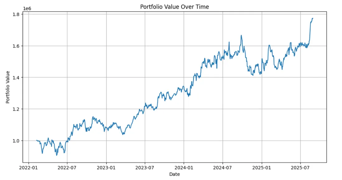Number of trading days: 880 Initial Funds: $1000000.00 Final Portfolio Value:$1774202.20 Maximum Drawdown: 15.34% Sharpe Ratio: 1.12 Final Percentage Return: 77.42%

Battle of the Algorithms: Choosing the Right Trading Brain When a quantitative firm decides to use Reinforcement Learning (RL), they aren’t just choosing an algorithm; they’re selecting a specific kind of AI brain, each optimized for different tasks and market behaviors. The fundamental choice boils down to a split between two architectural families: Value-Based (which map states to the expected reward) and Policy-Based (which develop a direct strategy).

1. The Value-Based Champion: DQN (Deep Q-Networks) DQN is the classic choice for teaching an agent to act optimally in simple, confined environments. It’s built on the concept of Q-Values (Quality-Values). DQN learns the Value (Q) of taking a specific, discrete action (e.g., Buy, Sell, Hold) in a specific state. This makes it excellent for simple trade execution where the action space is limited to a few clear choices. However, DQN fails entirely when actions are continuous (e.g., “Buy 42.7% of my capital,” “Sell 1,000,000 shares”). Therefore, it is not suitable for portfolio sizing or optimal execution tasks that require fine-grained control.

2. The Policy-Based Family: A2C, A3C, and PPO Policy-Based methods learn the Policy (the strategy or probabilities of actions) directly, making them essential for real-world trading that demands flexibility and continuous control.

A. A2C (Advantage Actor-Critic) & A3C The Actor-Critic structure is a major step up because it uses two separate neural networks working in tandem. The Actor (Policy) network decides what to do (e.g., Buy, Sell, or even the percentage to trade), functioning as the Trader who makes the decision. Separately, the Critic (Value) network estimates how good the Actor’s choice was compared to the baseline, acting as the Risk Manager. By having the Critic evaluate the Actor’s performance, the learning process is dramatically accelerated, as the Actor knows how much “better” (the Advantage) its action was, making A2C/A3C a powerful choice for dynamic, ever-changing markets.

B. PPO (Proximal Policy Optimization) — The Industry Champion PPO is currently the industry favorite and the default choice for modern, complex RL tasks in high-stakes environments like finance. PPO uses the Actor-Critic structure but adds a clever clip function to the policy update. This crucial feature prevents the Agent from taking a sudden, destructive step in its policy, thereby ensuring stable, predictable learning. Its stability and simplicity make it easier to tune and deploy successfully compared to rivals, making it highly reliable for continuous action spaces (e.g., fractional position sizing) and managing large, multi-asset portfolios.

While DQN was the starting pistol for deep RL in finance, PPO is the reigning champion for practical applications because it delivers the necessary stability and fine-grained, continuous control required to manage significant capital without risking catastrophic system errors.

Looking Ahead: What’s Next for RL in Trading The future of trading is defined by stability, explainability, and multi-agent competition. We are moving past the “black box” and toward a new paradigm where AI is required to be as rigorous and accountable as a human trader. By focusing on systems that learn continuously, understand causality, and integrate seamlessly into a market ecology of specialized agents, we are preparing for a future where intelligent systems manage risk and generate profit with unprecedented safety and verifiable logic. This shift represents the most exciting technological opportunity in modern finance.